Golden Ticket Exploration

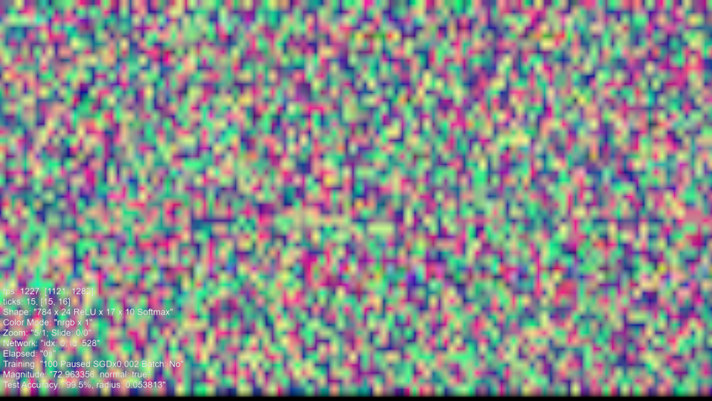
So, if we have made some network, initial state, not like this one:

And we applied typical backpropagation training process using SGDx0.002, on MNIST, we could get an image somehow like this:

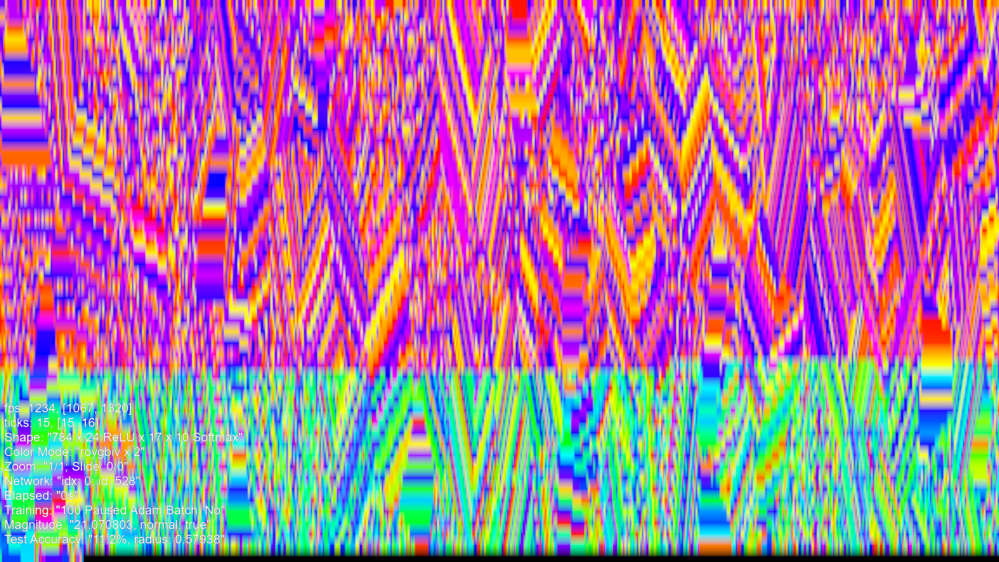
This is an image of a trained Golden Ticket than I created which is not Dyson Hatching and I will describe later.

What has happened? Like an eroding rock that gets shaped, the training process has shaped the network. However, instead of eroding, there is also much new growth. In the top image, the magnitude of the network is 22, and as a network trains, the magnitude goes up and down but gradually grows. At some point the network could obtain a high accuracy and this trained network has a magnitude of 72, and a 99.5% MNIST test accuracy. In theory, if trained more, depending on how, could potentially increase accuracy further, but in practice, is more likely to lose it (apparently overtraining). The magnitude will continue to go up and up, however.

Now, we have a lot of questions about these two images, and before that, I feel like I need to summarize what I’ve been doing for some years now, because it’s been quite odd.

So, I had been investigating networks in C++ and had been investigating algorithm experiments in backpropagation. At one point, the backpropagation math was broken, and I produced b-series networks, later I further modified it with an algorithm addition, and I produced series-c networks, both with an encoding I made called Curve Encoding, furthermore, both had very experimental training process. I then produced my Golden Ticket, idea and I removed my algorithm addition but still had broken math, even though ChatGPT didn’t notice how. Finally, after studying some python code on the internet with a newer ChatGPT: https://julianroth.org/documentation/neural_networks/basics.html

I produced correct backpropagation math. The problem had been that I was not saving and backpropagating the pre-activation and was rather using the activation.

The result is that network training became more effective, and I also wrote ADAM in addition to correct SGD, and started using Softmax. The algorithm additions and curve encoding are things I need to reinvestigate, but that’s on the TODO list. All of that is, of course, only part of the story – but that’s history.

So, these networks are images of Multi-Layered Perceptrons, or MLP. The top-left corner of the image is the first weight in the network, and the bottom ( toward right) row is part of the output layer. The image is of all the weights in the network, perceived as a single sequence of numbers, that can be ordered into a rectangle image.

The way I calculate the width and height of these images is as follows:

int width = firstSize * firstSize
, height = std::ceil(totalWeightSize / float(width));

where first size is the size of the first layer. So in a 24×17 network like above, the width of the rectangle is 24*24.

We place the pixels in the rectangle like so:

for (std::size_t y = 0; y < texBox.height; ++y) {
    for (std::size_t x = 0; x < texBox.width; ++x) {
        texBox.at(x, y) = mConvertedWeights[i]
        ++i;
    }
}

We can produce the above Dyston Hatching Golden Ticket by doing the following:

std::mt19937_64 random;
random.seed(528);

Next, the known algorithm can be called with: random, and vertexnum=256.

Now that we’ve can produce these images, it’s time to animate them with SDG and Adam, which of course is the next video.