Like I said earlier, this post is a sort of introduction to programming, however, it is not a typical, “Hello World” introduction. We’ll be using C++ and inline Assembly to investigate what exactly is going on in a program and C++. The following will be explained:
what a C++ program is and looks like to a computer
what variables are and how the stack and memory works
what functions are and how they work
how pointers work
how math and logic works, such as when you evaluate an equation
What a C++ program is and what it looks like to the computer
C++ and any programming language is just a bunch of words and syntax used to describe a process for the computer to perform.
You write a bunch of stuff, and the computer does exactly what you commanded it to. That said, while a program is a series of words and syntax to us, to the computer, it ends up being quite different. Computers only understand numbers, so somewhere between when a program is written and when it is executed by the computer, it gets interpreted from the programming language into numbers – Machine Code.
For example, the following program:
r = x + x * y / z - z * x
Looks like this in Machine Code:
Programming languages exist for a several reasons:
to provide an alternative to writing in Machine Code
to make writing maintainable and manageable code bases possible
to allow programmers to express themselves in different ways
to accomplish a task with efficiency given a language customized to that task
Finally, the basic C++ program that writes, “Hello World!”, to the console screen:
int main(){
 	std::cout << "Hello World!";
	return 0;
}
In Machine Code, it looks like this:
C++ is quite the improvement.
The language that translates closely to Machine Code is Assembly Language. While both Machine Code and Assembly Language are unpractical to work with, Assembly Language is actually something people do use, and we are going to use it to link what’s going on in the computer to what’s going on in C++.
Before we can move into Assembly, however, we need to review some basics of how programs work.
Memory
As we know, computers work with numbers, and a program is ultimately a bunch of numbers. The numbers are stored in the the computer in a place called memory, and lots of them, more numbers than you could count in your lifetime. It can be thought of as an array, grid or matrix where each cell contains a number and is a specific location in memory.
A visualization of memory.
These cells exist in sequence and that sequence describes its location. For instance, we could start counting memory at cell 1, and go to cell 7, and each of those locations could be referred to by their sequence number: 1 to 7.
The numbers in memory can represent one of two things:
a Machine Code or operand used to execute a command
some sort of Variable – an arbitrary value to be used by, or that has been saved by, a program
In programming languages such as C++, variables are referred to using names rather than their sequence number, and Machine Code is abstracted away with verbose language.
A snippet of C++ that declares three variables and prints them out.
The same snippet in Assembly; for glancing only.
The Stack: a type of Memory for Variables
Whenever a Variable is declared, it gets allocated in an area of Memory called the Stack. The Stack is a special type of Memory which is essential to how a C++ program executes. When a Variable enters scope, it gets allocated onto the Stack, and then later, when it exits scope, it’s removed from the Stack. The Stack grows in size as Variables enter scope and shrinks as Variables exit scope.
In C++, curly braces “{ “ and “ } “ are used to define a variable’s scope, also known as a block or epoch.
A C++ program with several blocks:
void main(){	//begin block a:

	//x is allocated, stack size goes to 1
	int x = 0;

	{	// begin block b:

		// k, l and m are allocated, stack size goes to 4
		int  k = 2,  l = 3, m = 4;

		// an example operation
		x = k + l + m;

	}	// end of block b, stack size shrinks back to 1

	// - back to block a - y is allocated, stack size goes to 2
	int y = 0;

	{	// begin block c:

		// l and o are allocated, stack size goes to 4
		int l = 12, o = 2;

		// an example operation
		y = l * o;

	}	// end of block c, stack size shrinks back 2

	// - back to block a - z is allocated, stack size goes to 3
	int z = 0;

	// an example operation
	z = x - y;

	// write result, z, to the console
	std::cout << z << std::endl;

}	// end of block a, stack shrinks to size 0
x86 Assembly Brief on the Stack
Assembly is really simple. Simple but lengthy and hard to work with because of its lengthiness. Lets jump right in.
A line of Assembly consists of a command and its operands. Operands are numbers of course, but these numbers can refer to a few different things: Constants ( plain numbers ), Memory locations (such as a reference to a Stack Variable), and Registers, which are a special type of Memory on the processor.
The Stack’s current location is in the esp register. The esp register starts at a high memory location, the top of the stack, such as 1000, and as it grows, the register is decremented, towards say, 900 and 500, and eventually to point where the stack can grow no further. General purpose registers include eax and are used to store whatever or are sometimes defaulted to with certain operations.
There are two commands that manipulate the stack implicitly:
push [operand]
put the operand value onto the Stack, and decrement esp
pop [operand]
remove a value from the Stack, store it in the operand register, and increment esp
Registers:
esp
the Stack’s top, moves up or down depending on pushes/pops, or plain adds/subtracts.
eax
a general purpose register
Given these two instructions we can create and destroy stack variables. For instance, similar to the program above but without the example equations:
_asm{

	push 0		//create x, with a value of 0

	push 2		//create k
	push 3		//create l
	push 4		//create m
	//do an equation
	pop eax		//destroy m
	pop eax		//destroy l
	pop eax		//destroy k

	push 0		//create y

	push 12		//create l
	push 2		//create o
	//do an equation
	pop eax		//destroy o
	pop eax		//destroy l

	push 0		//create z
	//do an equation

	pop eax		//destroy z
	pop eax		//destroy y
	pop eax		//destroy x
}
Another way to manipulate the Stack/esp involves adding or subtracting from esp. There is an offset in bytes which is a multiple of the Stack alignment, on x86, this is 4 bytes.
add esp, 12 	// reduce the stack by 12 bytes – same as 3 * pop
sub esp, 4 	// increase the stack by 4 bytes – same as 1 * push
The difference in usage is that add and sub do not copy any values around. With add, we trash the contents, and with sub, we get uninitialized space.
Once Stack space has been allocated, it can be accessed through dereferencing esp. Dereferencing is done with brackets.
[esp]  		// the top of the stack, the last push
[esp + 4] 	// top + 4 bytes, the second to last push
[esp + 8] 	// top + 8 bytes, the third to last push
//[esp – x ] 	makes no sense
Adding in the example equations requires some additional commands:
add [add to, store result], [ operand to add ]
adds the operand to register
sub [subract from, store result], [ operand to subtract ]
subtracts the operand from the register
mul[operand to multiply by eax, store in eax ]
multiplies the operand by the eax register
mov [ copy to ], [ copy from ]
copies a value from a Register to Memory or vice versa.
_asm{

	push 0			//create x, with a value of 0

	push 2			//create k
	push 3			//create l
	push 4			//create m

	//k + l + m;
	mov eax, [esp + 8]	// copy k into eax
	add eax, [esp + 4] 	// add l to eax
	add eax, [esp]		// add m to eax

	add esp, 12		//destroy k through m

	//store the value in x
	mov [esp], eax

	push 0			//create y

	push 12			//create l
	push 2			//create o

	// l * o
	mov eax, [esp + 4]	 //copy l into eax
	mul [esp]		 //multiply o by eax

	add esp, 8		//destroy l and o

	//store the value in y
	mov [esp], eax

	push 0			//create z

	//x - y;
	mov eax, [esp + 8]
	sub eax, [esp + 4]

	mov [esp], eax		//write to z; z = -15

	add esp, 12		//destroy z through x

}
Functions
Functions are a way to associate several things:
A Stack block
Code
A useful name
As we know, rather than writing out the same code over and over, to reuse it, we can use a function.
But that is not the end of what functions are, they are also Named Code Segments, a segment of code with has a useful name, a name that both describes what the function does, and that be used to call that function in the language.
In C++ functions have four properties:
return type
function name
parameters
function body
And the following prototype:
[return type] [name]([parameters]){[body]}
In C++ a sum function would look like so:
int sum( int x, int y ){
	return x + y;
}
In assembly to sum these two values we’d do the following:
push 5 			// y = 5
push 4 			// x = 4
mov eax, [esp] 		//eax = x
add eax, [esp+4]	//eax = 9
add esp, 8		//clear stack
You can see there are three stages here:
Setting up the function’s parameters using push
the actual function code
resetting the stack
We are also missing three things, the function name, the return type, and actually calling the function. In assembly, a function name is the same as a C++ label:
sum:
Now comes an interesting part – assembly – since we can do anything in it, is going to implement something called a: Calling Convention – how the function’s parameters are passed, how the stack is cleaned and where, and how the return value is handled.
In C++ the default calling convention is called cdecl. In this calling convention, arguments are pushing onto the stack by the caller, and in right to left order. Integer return values are saved in eax, and the caller cleans up the stack.
First off, to actually call a function we could use a command, jmp. Jmp is similar to the C++ goto statement. It sends the next instruction to be processed to a label. Here’s how we could implement a function using jmp:
_asm{

	jmp main

sum:		//sum function body
	mov eax, [esp+4]	//we have a default offset due to the return address
	add eax, [esp+8]
	jmp [esp]		//return to: sumreturn

main:		//main program body
	push 5			//we plan to call sum, so push arguments
	push 4
	push sumreturn		//push the return address
	jmp sum			//call the function

sumreturn:
	add esp, 12		//clean the stack
	//result is still in eax
}
To make this much easier, there are additional instructions:
call [operand]
automatically pushes the return address onto the stack and then jumps to the function
ret [ optional operand ]
automatically pops the return address and jumps to it
These instructions wrap up some of the requirements of function calling – the push/pop of the return address, the jmp instructions, and the return label. With these additional instructions we’d have the following:
_asm{

	jmp main
sum:
	mov eax, [esp+4]	//we have a default offset due the to return address
	add eax, [esp+8]
	ret
main:
	push 5			//we plan to call sum, so push arguments
	push 4
	call sum

	add esp, 8		//clean the stack
	//result is still in eax
}
In other calling conventions, specifically x64 ones, most parameters are passed in registers instead of on the stack by default.
With cdecl, every time we call sum, we have an equivalent assembly expansion:
push 5			//pass an argument
push 4			//pass an argument
call sum		//enter function
add esp, 8		//clear arguments
Recursive functions run out of stack space if they go too deep because each call involves allocations on the stack and it has a finite size.
Pointers
Pointers confuse a lot of folks. What I think may be the source of the confusion is that a pointer is a single variable with two different parts to it, and indeed, a pointer is in fact its own data type. All pointers are of the same data type, pointer. They all have the same size in bytes, and all are treated the same by the computer.
The two parts of a pointer:
The pointer variable itself.
The variable pointed to by the pointer.
In C++, non-function pointers have the following prototype:
[data type]* [pointer variable name];
So we actually have a description of two different parts here.
The Data Type
this is the type of the variable that is pointed to by the pointer.
The Pointer Variable
this is a variable which points to another variable.
What a lot of folk may not realize, is that all Dynamic Memory ultimately routes back to some pointer on the Stack, and to some pointer period – if it doesn’t, that Dynamic Memory has been leaked and is lost forever.
Consider the following C++
int* pi = new int(5);
With this statement, we put data into two different parts of memory; the first part is the Stack, it now has pi on it, the second, int(5), is on the heap. The value contained by the pi variable is the address of int(5). To work with a value that is pointed-to by a pointer, we need to tell the computer to go and fetch the value at the pointed-to address, and then we can manipulate it. This is called Dereferencing.
int i = 10;		//declare i on the stack
int* pi = &i;		//declare pi on the stack and set it's value to the
 			//address of i
*pi = *pi + 7;		//dereference pi, add 7, assign to i
 // i = 17
So in assembly, there is an instruction used to Dereference:
lea [operand a ] [operand b]
Load Effective Address, copy b into a
lea a, value performs the following process:
stores value in a
such that
lea eax, [ eax + 1] will increment eax by 1
and
lea eax, [ esp + 4 ] takes the value of esp, an address, adds 4, and stores it in eax
_asm {

	//initialization
	push 10			//a value, i
	push 0			//a pointer, pi

	lea eax, [esp + 4]	//store the address of i in eax
	mov [esp], eax		//copy the address of i into pi

	//operations
	mov ebx, [esp] 		//dereference esp, a value on the stack, and get the value
 				//of pi - the address of i
	add [ebx], 7		//dereference pi and add 7, i == 17

	//[esp+4] now == 17

	add esp, 8		//clean the stack
}
So these examples pointed to memory on the stack, but the same process goes for memory on the heap as well, that memory is just allocated with a function rather than push.
Logic and Math
Probably the key aspect of programming is the use of if-statements. Anif-statement can be a long line of code and obviously that means it turns into lots of assembly statements. What you may not realize though, is that a single C++ if-statement actually often turns into multiple assembly if-statements. So lets examine what an if-statement is in assembly.
Consider the following C++:
int x = 15;
if( x == 10 ) ++x;
Can result in the following assembly:
_asm {

	push 15 // x

	cmp [esp], 10		//compare x with 10 and store a comparison flag.
	jne untrue		//jump to a label based on the comparison flag.
				//in this case, ne, jump if not-equal.
				//since 15 != 10, jump to untrue and skip the
  				//addition. If x was 10, it would be executed.

	add [esp], 1		//increment x by 1
untrue:
	//proceed whether it was evaluated true or not
	add esp, 4		//clean stack
}
If–statements generate multiple jumps when there are logical operators in the statement. This results in an if-statement property called short-circuiting. Short Circuiting is a process in which only some of the if-statement may be executed. In the case where the first failure of a logical operation evaluates the if-statement as false, the subsequent logical operations are not evaluated at all.
An example of and logical operator:
int x = 10, y = 15;
if( x == 10 && y == 12) ++x;
_asm {

	push 10 // x
	push 15 // y

	//the first statement
	cmp [esp+4], 10			//if the current logic operation evaluates
 	jne untrue			//the statement to false, then all other
 					//operations are skipped.
					//in our case it was true so we continue to
 	//the second statement
	cmp [esp], 12			//this comparison is false, so we jump
	jne untrue

 	//only evaluated if both and operands were true
	add [esp+4], 1			//increment x by 1
untrue:
	//proceed whether it was evaluated true or not
	add esp, 8			//clear stack
}
In the above example, if x had been != 10, then y == 12 would not have been evaluated.
An example with the or logical operator.
int x = 10, y = 15;
if( x == 10 || y == 12) ++x;
_asm {
	push 10 // x
	push 15 // y

	cmp [esp+4], 10
	je true				//if the first statement is true, no need to
 					//evaluate the second

	cmp [esp], 12			//if the first statement evaluated false,
	jne untrue			//check the next statement

true:
 	//evaluated if either or operand was true
	add [esp+4], 1			//increment x by 1
untrue:
	//proceed whether it was evaluated true or not
	add esp, 8			//clear stack
}
Logical order of operations is going to be left to right order, which ensures that sort circuiting works as expected.
Back to the top, we had the following equation:
r = x + x * y / z - z * x
This entire equation needs to be evaluated, and as you realize, this is a bunch of assembly steps. The order in which the steps execute is almost certainly not left to right, but is some sort of logical order-of-operations which is also optimized to be speedy and effecient.
The equation has four steps:
a = + x*y/z
b = + x
c = + z*x

result = a + b  - c
Again, the order is going to respect mathematical order of operations, and try to run efficiently on the computer. Here’s how it may turn out:
_asm {

	//setup
	//all of these variables are integers and the operations are integer
	push 10	//x
	push 15	//y
	push 2		//z

	//cache x its used 3 times: ebx = x
	mov ebx, [esp+8]

	//eax = x*y/ z
	mov eax, ebx
	mul [esp+4]
	div [esp]

	//ecx = eax + x
	add eax, ebx
	mov ecx, eax

	//eax = ez*ex
	mov eax, [esp]
	mul ebx

	//finally, subtract: perform ( ex*ey/ez + ex ) - (ez*ex) = ecx
	sub ecx, eax

	//result is in ecx

	add esp, 12		//clear stack
}
On a final note, if you want to get output from these examples into c++, here’s an easy way for Visual Studio:
int main(int argc, char**argv){

	int result =0;

	_asm{
		mov eax, 5
		mov dword ptr[result], eax
	}

	std::cout << result;
	std::cin.get();

	return 0;
}
That’s it for this post! In the future I’ll mostly post about C++ programming itself. I would love to hear your comments below! Good Luck!
I followed RaffK project to its completion and did much more feature development such as complete chat feature. I created a lot of Modern and screaming Future C++, it is sort of crazy. This ChatGPT2 animation experiment involved training chatgpt2 on scrolling Shakespeare 1000 times using SGD with a learn rate of 0.0002. After SGD has updated the weights/bias, I record a subsection of GPT2 Tensors to file. The file generated is about 2GB and contains 1000 frames of chatgpt2 data.
In another project, Float Space Animator, is able to view and convert Float Spaces in real-time interface. This was used to create three programs, an animation of std::mt19937, a to view of ChatGPT2 Tensor Space (weights/bias), and also, an animation ChatGPT2 by showing each saved ChatGpt2 frame in sequence at 7 frames per second.
The Animator project has a windows release on github. It can be easily changed to another OS because I use SDL and OpenGL which are portable. At some point, I plan to create an Apple release.
Future Animator work is going to be a project to view .fits files.
Now that the ChatGPT2 portion of my project seems to be complete, the next phase of NetworkLib, is to recreate my old work using my new abilities and in an open-source format. This will allow real-time animations of relatively small MLP, and I am curious of NVIDIA performance enhancements for larger MLP.
This will involve training MNIST and will animate MNIST at least.
Future ChatGPT2 work would include using the larger models and training from scratch. I am going to make an animation of the Activation Space Tensor, rather than the weights/bias, which is the current ChatGPT2 animation.
There are so many C++ concepts that are straight from the future, and they keep arriving at a rapid pace. One plan for the MLP animator is to develop mdspan in my Tensor object and perhaps change Tensor a lot.
One of the most interesting new features is std::views::zip and how it changes the expression of math.
There are two ways to write this in Modern C++, for two-parameters, you could use transform, or for n-many parameters, there is zip. Both of these ways express the math in a new way.
std::transform(output.begin(), output.end(), weights.begin(), output.begin(), [in](auto o, auto w) {
return o + w * in;
});
With transform, the limit is two parameters, but with zip, there can be many, and the code is much cleaner, it is easy to cope with the Future in this case:
for (const auto& [o, w] : std::views::zip(output, weights))
	o += w * in;
It is hard to believe that mathematics gets more complicated than two parameters but when it does, it now looks pretty good.
This could be done with two transforms, a lot of i’s, or one zip.
for (const auto& [q, dq, k, dk] : std::views::zip(qh, dqh, kh, dkh)) {

	dq += o * k;
	dk += o * q;
}
This code is used in linear normalization:
float norm = 0;
for (const auto& [i, w, b, o] : std::views::zip(in, weight, bias, out)) {
	norm = (i - mean) * r_stdDev;
	o = norm * w + b;
}
The C/C++ loop has been left in the dust by ever advancing range and view based loops, i-loops look much worse and will soon be old code smell.
These zip loops are basically ranged based loop introduced in C++11.
for( const auto& i : in ) // a single range
for( const auto& [ a, b ] : std::views::zip(as, bs) // two ranges
The way ranges and views can be iterated over, can altered, using | operator.
for( const auto& i : in | std::views::reverse )
There are lots of cool | features and transforms for ranges and views and I expect this operator to become super common in Modern/Future C++, so it should be on your C++ radar if it isn’t.
for(const auto& text : document | std::views::slide(size) )
In this code, we iterate over document, by sliding across it with a size chunk. I considered this code when fetching the training data for ChatGPT2, but I decided the step size of 1 was unacceptable, and went with another method.
The loop-i is sometimes necessary, in this case there is iota_view
for( const auto& i : std::views::iota(0, 1000))
In this case, we see: i, begin index, and size. No equality expressions or increments here. We do future code like so for some reason:
for( const auto& i : std::views::iota(0, 1000) | std::views::reverse)
A normal C/C++ reverse loop is a good way to look like a C programmer from decades past, and that’s super old in 2025.
At this point there is a clear departure from code that is in the standard library and projects not based on the library. Projects not based on the library have lost access to ever advancing C++ programming expressions and constructs. Projects from the library are becoming so advanced and different, that soon C++ will be as different, from C/C++ is from C, and even much more different.
Right now, ChatGPT2 forwards and produced output prediction. Seems really amazing, except there seems to be a problem — the output begins to repeat very quickly.
The tail of the first 1024 tokens of the test text, looks like so:
First Citizen: Care for us! True, indeed! They ne’er cared for us yet: suffer us to famish, and their store-houses crammed with grain; make edicts for usury, to support usurers; repeal daily any wholesome act established against the rich, and provide more piercing statutes daily, to chain up and restrain the poor. If the wars eat us not up, they will; and there’s all the love they bear
Concerning First Citizen, here is what ChatGPT2 124 proceeds to write:
for us, and the poverty they have to endure.
First Citizen:
We are not to be taken for fools, but for the people.
Second Citizen:
We are not to be taken for fools, but for the people.
MENENIUS:
What do you mean, what do you mean?
[repeats from First Citizen point for a continuous sequence of 3]
It seems to quickly repeat given input data, and the question is: error or not? It sure seems strange, to repeat…
I am working to understand GPT2 more right now and additionally working to understand Raff K code better, to help identify the source of the error if there is one. There is also a project by karpathy that I am thinking to reference before long.
I kind of feel like there could be a major problem with what I’ve written and it is quite concerning! However, the project persists…
Since C++ 20, there are Future C++ people creating sum functions that are coroutines. C++20 introduces new keywords such as co_await, co_yield, and co_return, and much more in support of a new feature called coroutines, which is a way to pause a function and run some other function, only to return later while that other function has paused itself.
With multiples of these objects, it is possible to experience asynchronisticy but without actually working with threading, this is a new C++ paradigm.
So, if we have made some network, initial state, not like this one:
And we applied typical backpropagation training process using SGDx0.002, on MNIST, we could get an image somehow like this:
This is an image of a trained Golden Ticket than I created which is not Dyson Hatching and I will describe later.
What has happened? Like an eroding rock that gets shaped, the training process has shaped the network. However, instead of eroding, there is also much new growth. In the top image, the magnitude of the network is 22, and as a network trains, the magnitude goes up and down but gradually grows. At some point the network could obtain a high accuracy and this trained network has a magnitude of 72, and a 99.5% MNIST test accuracy. In theory, if trained more, depending on how, could potentially increase accuracy further, but in practice, is more likely to lose it (apparently overtraining). The magnitude will continue to go up and up, however.
Now, we have a lot of questions about these two images, and before that, I feel like I need to summarize what I’ve been doing for some years now, because it’s been quite odd.
So, I had been investigating networks in C++ and had been investigating algorithm experiments in backpropagation. At one point, the backpropagation math was broken, and I produced b-series networks, later I further modified it with an algorithm addition, and I produced series-c networks, both with an encoding I made called Curve Encoding, furthermore, both had very experimental training process. I then produced my Golden Ticket, idea and I removed my algorithm addition but still had broken math, even though ChatGPT didn’t notice how. Finally, after studying some python code on the internet with a newer ChatGPT: https://julianroth.org/documentation/neural_networks/basics.html
I produced correct backpropagation math. The problem had been that I was not saving and backpropagating the pre-activation and was rather using the activation.
The result is that network training became more effective, and I also wrote ADAM in addition to correct SGD, and started using Softmax. The algorithm additions and curve encoding are things I need to reinvestigate, but that’s on the TODO list. All of that is, of course, only part of the story – but that’s history.
So, these networks are images of Multi-Layered Perceptrons, or MLP. The top-left corner of the image is the first weight in the network, and the bottom ( toward right) row is part of the output layer. The image is of all the weights in the network, perceived as a single sequence of numbers, that can be ordered into a rectangle image.
The way I calculate the width and height of these images is as follows:
so now it is time to make use of the voronoi diagram. To begin, I want to calculate the average slope of the edges of each cell
ChatGPT:
The slope of a line is typically calculated as the difference in the y-coordinates of two points divided by the difference in the x-coordinates of those two points. Given two points P1(x1, y1) and P2(x2, y2), the slope of the line between them is given by:
slope = (y2 – y1) / (x2 – x1)
Keep in mind that this formula does not work if x1 equals x2, as this would mean you’re dealing with a vertical line. In this case, the slope is usually said to be undefined or infinite.
For a Voronoi cell, you can calculate the slope of each edge by applying this formula to each pair of adjacent vertices in the cell. Here’s an idea of how to proceed:
Iterate through each Voronoi cell in your Voronoi diagram.
For each cell, iterate through each pair of adjacent vertices. Note that you will have to treat this list of vertices as cyclic to make sure you also get the edge between the last and first vertex in the list.
Calculate the slope of the edge between each pair of adjacent vertices using the formula above.
Add these slopes up and then divide by the number of edges to get the average slope for the cell.
Here’s some pseudo-code for this process:
for each cell in voronoi.cells:
    total_slope = 0
    for i in range(len(cell.vertices)):
        // Get the current vertex and the next vertex in the list
        // (or the first vertex if we're at the end of the list)
        v1 = cell.vertices[i]
        v2 = cell.vertices[(i+1) % len(cell.vertices)]

        // Calculate the slope of the edge between v1 and v2
        // (we're assuming here that v1.x != v2.x)
        slope = (v2.y - v1.y) / (v2.x - v1.x)

        // Add the slope to the total slope
        total_slope += slope

    // Calculate the average slope for the cell
    average_slope = total_slope / len(cell.vertices)
This will give you the average slope of the edges for each cell. Note that this is a kind of “net” average slope, considering the direction of each edge.
Nick:
Here’s what I did:
             std::for_each(std::execution::par, cells.begin(), cells.end(), [&](auto& cell) {

                float totalSlope = 0;
                for (std::size_t i = 0; i < cell.vertices.size(); ++i) {
                    // Get the current vertex and the next vertex in the list
                    // (or the first vertex if we're at the end of the list)
                    auto& v1 = cell.vertices[i];
                    auto& v2 = cell.vertices[(i + 1) % cell.vertices.size()]; //perform loop of poly

                    float slope = 0;
                    auto d = v2.x - v1.x;
                    if (d != 0)
                        slope = (v2.y - v1.y) / d;
                    else //fudge slope
                        slope = 10000;

                    // Add the slope to the total slope
                    totalSlope += slope;
                }

                cell.slope = totalSlope / cell.vertices.size();
                });
ChatGPT:
Your code looks correct. It follows the process I described earlier.
You’re correctly handling the case where the denominator of the slope calculation could be zero (which would happen if an edge is vertical), and you’re using a high “fudge” value for the slope in this case. This value effectively represents an “infinite” slope, which is a reasonable choice.
Just keep in mind that the “net” average slope value you’re calculating won’t necessarily give you a representative measure of how steep the slopes of the cell’s edges are. It takes into account the direction of each edge, so if some edges have positive slope and others have negative slope, they could cancel each other out in the average.
If you want to measure the steepness of the slopes regardless of their direction, you could take the absolute value of each slope before adding it to the total. This would give you an average of the absolute values of the slopes, which might be more useful in some applications.
In general, the approach you’re taking is correct for calculating the average slope of the edges in each Voronoi cell.
Nick:
the absolute value is a good addition
ChatGPT:
I’m glad you found the suggestion useful! Using the absolute value can provide a more meaningful measurement in many cases, especially when you’re interested in the magnitude of the slope rather than its direction. Just keep in mind that this does lose some information about the directionality of the slopes, so choose the method that best suits your specific needs.
Here’s the modified code snippet:
std::for_each(std::execution::par, cells.begin(), cells.end(), [&](auto& cell) {
    float totalSlope = 0;
    for (std::size_t i = 0; i < cell.vertices.size(); ++i) {
        // Get the current vertex and the next vertex in the list
        // (or the first vertex if we're at the end of the list)
        auto& v1 = cell.vertices[i];
        auto& v2 = cell.vertices[(i + 1) % cell.vertices.size()]; //perform loop of poly

        float slope = 0;
        auto d = v2.x - v1.x;
        if (d != 0)
            slope = std::abs((v2.y - v1.y) / d);
        else //fudge slope
            slope = 10000;

        // Add the absolute slope to the total slope
        totalSlope += slope;
    }

    cell.slope = totalSlope / cell.vertices.size();
});
This modification uses the std::abs function to compute the absolute value of the slope before adding it to totalSlope. As a result, the cell.slope value will represent the average steepness of the cell’s edges, regardless of their direction.
Nick:
So these cells are going to be drawn using pixels on the screen. I want to fill each cell with lines of their given slope.
ChatGPT:
To accomplish that, you can use Bresenham’s line algorithm for each cell, which draws a line between two points in a grid of discrete cells, such as pixels on a screen. The algorithm uses integer operations only, which makes it very efficient.
Given the set of points defining the boundary of a Voronoi cell, we can draw the cell by drawing lines between each pair of consecutive points. Once we have the boundary, we can fill the cell with lines of the given slope.
Here’s a basic idea of how you might implement that:
// The function to draw a line between two points using Bresenham's line algorithm
void drawLine(Vertex start, Vertex end, float slope, ScreenBuffer& buffer) {
    // ... Implementation of Bresenham's line algorithm here ...
    // ... Depending on the slope, draw lines inside the cell ...
}

// Then, for each cell:
for (const auto& cell : cells) {
    // Draw the boundary of the cell
    for (std::size_t i = 0; i < cell.vertices.size(); ++i) {
        auto& v1 = cell.vertices[i];
        auto& v2 = cell.vertices[(i + 1) % cell.vertices.size()];
        drawLine(v1, v2, cell.slope, buffer);
    }
}
You’ll have to adjust this to match your actual code and data structures, of course. Also, filling a cell with lines of a given slope is a non-trivial task which will require a careful implementation. One approach could be to first draw the boundary of the cell, then repeatedly draw lines of the given slope across the cell, starting from different points on the boundary.
Note: Be aware that graphical rendering is beyond the capabilities of standard C++. You’ll need to use a graphics library that provides a way to draw individual pixels on the screen, like SDL or SFML. The ScreenBuffer in the example above would be something provided by your graphics library that you can draw to.
Nick:
So, we will need to first identify a rectangle which contains the polygon, then, for each x pixel in the rect length, identify the top and bottom y boundaries from the polygon, and then, using the rect, which I filled with lines of the given slope previously, I can identify the pixel color of the poly pixel
ChatGPT:
Yes, that’s a good plan!
For each cell, calculate a bounding rectangle. The simplest way to do this is to find the minimum and maximum x and y coordinates of the vertices of the cell.
For each x position within this bounding rectangle, calculate the intersections of a vertical line at that x position with the cell. This will give you the top and bottom y boundaries for that x position.
Create an offscreen buffer for the rectangle and fill it with lines of the given slope.
For each y position between the top and bottom boundaries, take the color of the corresponding pixel from the offscreen buffer and use it to fill the cell on your main screen buffer.
Here is some pseudo code that summarizes the steps:
for (const auto& cell : cells) {
    // Calculate bounding rectangle
    auto [minX, maxX, minY, maxY] = calculateBoundingRectangle(cell);

    // Create offscreen buffer and fill it with lines of the given slope
    ScreenBuffer offscreenBuffer(maxX - minX, maxY - minY);
    fillBufferWithLines(offscreenBuffer, cell.slope);

    // For each x position within the bounding rectangle
    for (int x = minX; x < maxX; ++x) {
        // Calculate top and bottom y boundaries
        auto [topY, bottomY] = calculateYBoundaries(cell, x);

        // For each y position between the top and bottom boundaries
        for (int y = topY; y < bottomY; ++y) {
            // Get color from offscreen buffer
            auto color = offscreenBuffer.getPixel(x - minX, y - minY);

            // Draw pixel on main screen buffer
            mainScreenBuffer.setPixel(x, y, color);
        }
    }
}
Please note that this is a rough pseudo-code and you would need to adapt this to fit your specific program structure. Also note that the function names used in this example are descriptive and need to be implemented according to your needs. The exact details of how to do this will depend on which graphics library you are using.
Nick:
So for the line filling, each pixel across the top of the bounding recangle will correspond to a striped line the color of which is random
ChatGPT:
Here is a possible approach to achieve this:
Generate the color for each pixel at the top of the bounding rectangle randomly.
For each x position within the bounding rectangle, determine the start and end points for the stripe line based on the slope.
Use the color for the corresponding x position at the top to draw a line from the start point to the end point in the offscreen buffer.
This approach assumes that you have functions or methods to generate random colors and to draw lines in your offscreen buffer. If you’re using an image manipulation library, you might find built-in functions for these tasks.
Here is a pseudocode example:
// Create offscreen buffer and fill it with lines of the given slope
ScreenBuffer offscreenBuffer(maxX - minX, maxY - minY);

for (int x = 0; x < offscreenBuffer.getWidth(); ++x) {
    // Generate a random color for this x position
    Color color = generateRandomColor();

    // Determine the start and end points for the stripe line
    Point startPoint(x, 0);
    Point endPoint(x + cell.slope * offscreenBuffer.getHeight(), offscreenBuffer.getHeight());

    // Draw the line in the offscreen buffer using the generated color
    offscreenBuffer.drawLine(startPoint, endPoint, color);
}
This code will draw a series of colored lines in the offscreen buffer, each line starting from an x position at the top of the buffer and extending downward at an angle determined by the cell’s slope. This will create a striped pattern in the buffer. Note that the generateRandomColor() function should return a random color, and the drawLine() method should draw a line from startPoint to endPoint in color.
When you then transfer the pixels from the offscreen buffer to your main screen buffer, each cell will be filled with a pattern of colored lines that match the cell’s average slope.
Again, this is rough pseudocode, so you’ll need to adjust it to fit your specific program and graphics library. For instance, if your graphics library uses a different origin point or coordinate system, you’ll need to adjust the line calculations accordingly.
Nick:
actually, using this method, parts of the polygon area may not have been filled with lines, for instance if the slope of the line was 45 degrees, then there will be a region of the rectangle that was not filled with lines
ChatGPT:
You’re right, and that’s a good observation. For steep slopes, a stripe pattern drawn from left to right won’t cover the entire rectangle. There are a couple of ways you could address this:
Always draw stripes in the direction that maximizes coverage. This means that if the slope of a cell is less than 1 (or -1), draw the stripes vertically (from top to bottom), otherwise draw them horizontally (from left to right). This guarantees that the stripes will cover the entire rectangle.
Alternatively, you could draw the stripes from one corner of the rectangle to the opposite corner, rather than from top to bottom or left to right. This way, the stripes would always cover the entire rectangle, regardless of their slope.
Here’s an adjusted pseudocode example for the first approach:
// Create offscreen buffer and fill it with lines of the given slope
ScreenBuffer offscreenBuffer(maxX - minX, maxY - minY);

if (abs(cell.slope) < 1) {
    // If the slope is less than 1, draw the stripes vertically
    for (int x = 0; x < offscreenBuffer.getWidth(); ++x) {
        // Generate a random color for this x position
        Color color = generateRandomColor();

        // Determine the start and end points for the stripe line
        Point startPoint(x, 0);
        Point endPoint(x, offscreenBuffer.getHeight());

        // Draw the line in the offscreen buffer using the generated color
        offscreenBuffer.drawLine(startPoint, endPoint, color);
    }
} else {
    // If the slope is greater than or equal to 1, draw the stripes horizontally
    for (int y = 0; y < offscreenBuffer.getHeight(); ++y) {
        // Generate a random color for this y position
        Color color = generateRandomColor();

        // Determine the start and end points for the stripe line
        Point startPoint(0, y);
        Point endPoint(offscreenBuffer.getWidth(), y);

        // Draw the line in the offscreen buffer using the generated color
        offscreenBuffer.drawLine(startPoint, endPoint, color);
    }
}
And here’s a pseudocode example for the second approach:
// Create offscreen buffer and fill it with lines of the given slope
ScreenBuffer offscreenBuffer(maxX - minX, maxY - minY);

// Calculate the length of the diagonal of the rectangle
int diagonalLength = sqrt(offscreenBuffer.getWidth() * offscreenBuffer.getWidth() + offscreenBuffer.getHeight() * offscreenBuffer.getHeight());

for (int d = 0; d < diagonalLength; ++d) {
    // Generate a random color for this position along the diagonal
    Color color = generateRandomColor();

    // Determine the start and end points for the stripe line
    Point startPoint(d, 0);
    Point endPoint(0, d);

    // Draw the line in the offscreen buffer using the generated color
    offscreenBuffer.drawLine(startPoint, endPoint, color);
}
Again, these are rough pseudocode examples, so you’ll need to adjust them to fit your specific program and graphics library.
Nick:
I think the solution is that for each empty pixel, create a line given y=mx+b, and then some series of pixels will become non-empty, and then repeat this process
ChatGPT:
Yes, that’s a feasible solution. If the cell’s bounding rectangle has empty pixels after filling with lines based on the slope, you can find each empty pixel, create a line from that point using the equation y = mx + b with the given slope, until no more empty pixels are found.
Here’s a high-level pseudocode to describe the procedure:
// Fill buffer with lines of given slope until no more empty pixels
while (there are empty pixels in the bounding rectangle) {
    for each pixel in the bounding rectangle {
        if (pixel is empty) {
            // Determine the line equation using the pixel's x-coordinate and the cell's slope
            float y = cell.slope * pixel.x + b;

            // Calculate the points for the new line
            Point startPoint(pixel.x, y);
            Point endPoint(pixel.x + 1, y + cell.slope);

            // Draw the line in the buffer using the color corresponding to the current pixel
            offscreenBuffer.drawLine(startPoint, endPoint, pixel.color);
        }
    }
}
In this pseudocode, b is the y-intercept of the line which you would need to calculate for each line you draw. You might adjust it based on the particular pixel position. Please note that this is a general guide and may require adjustments based on the specifics of your implementation.
Nick:
what is the code to test a line segment to see if it contains an x value
ChatGPT:
If you have a line segment defined by two points (x1, y1) and (x2, y2), you can determine whether the line segment contains a certain x value, say x0, by simply checking if x0 is within the range of x1 and x2.
Here’s a simple C++ function that does the check:
bool lineSegmentContainsX(const float x1, const float x2, const float x0) {
    // Determine the min and max x values of the line segment
    float minX = std::min(x1, x2);
    float maxX = std::max(x1, x2);

    // Check if x0 is within the range of the line segment
    return (x0 >= minX && x0 <= maxX);
}
This function checks whether the provided x0 value falls within the range of the line segment defined by x1 and x2. It will return true if x0 is between x1 and x2, and false otherwise. Please note that this assumes the line segment is a straight line along the x-axis. If the line is not straight, then this calculation would be insufficient.
Nick:
ok to determine the y values for a given x, i wrote this:
ChatGPT:
Apologies, but it seems you didn’t provide any code in your last message. Could you please provide the code you wrote so I can review it?
Nick:
            std::array<float,2> getPolyYBounds( float x) {

                std::vector<float> boundY; boundY.reserve(2);

                for (std::size_t i = 0; i < vertices.size(); ++i) {

                    auto& v1 = vertices[i];
                    auto& v2 = vertices[(i + 1) % vertices.size()]; //perform loop of poly

                    float minX = std::min(v1.x, v2.x);
                    float maxX = std::max(v1.x, v2.x);

                    // Check if x0 is within the range of the line segment
                    if (x >= minX && x <= maxX) {
                        float d = v2.x - v1.x;
                        float y = 0;
                        if (d != 0) {
                            float m = (v2.y - v1.y) / d;
                            y = m * x + v1.x;
                        }
                        boundY.push_back(y);
                        if (boundY.size() == 2) break;
                    }
                }
                return { boundY.front(), boundY,back() };
            }
ChatGPT:
Your code seems correct in identifying the range of y values for a given x along the boundary of the polygon. However, the computation of y seems to be incorrect. The correct way to compute y should be y = m * (x - v1.x) + v1.y;.
Here is the corrected code:
std::array<float,2> getPolyYBounds(float x) {

    std::vector<float> boundY;
    boundY.reserve(2);

    for (std::size_t i = 0; i < vertices.size(); ++i) {

        auto& v1 = vertices[i];
        auto& v2 = vertices[(i + 1) % vertices.size()]; //perform loop of poly

        float minX = std::min(v1.x, v2.x);
        float maxX = std::max(v1.x, v2.x);

        // Check if x is within the range of the line segment
        if (x >= minX && x <= maxX) {
            float d = v2.x - v1.x;
            float y = 0;
            if (d != 0) {
                float m = (v2.y - v1.y) / d;
                y = m * (x - v1.x) + v1.y;
            }
            boundY.push_back(y);
            if (boundY.size() == 2) break;
        }
    }
    return { boundY.front(), boundY.back() };
}
I’d also recommend checking if boundY actually contains two elements at the end of the function, because it’s possible for boundY to contain less than two elements if the x value doesn’t intersect with any line segments of the polygon. If boundY doesn’t contain two elements, you may want to handle this case appropriately, either by returning an error or by providing default values.
Nick:
            std::vector<float> getPolyYBounds( float x) {

                std::vector<float> boundY; boundY.reserve(2);

                for (std::size_t i = 0; i < vertices.size(); ++i) {

                    auto& v1 = vertices[i];
                    auto& v2 = vertices[(i + 1) % vertices.size()]; //perform loop of poly

                    float minX = std::min(v1.x, v2.x);
                    float maxX = std::max(v1.x, v2.x);

                    // Check if x0 is within the range of the line segment
                    if (x >= minX && x <= maxX) {
                        float d = v2.x - v1.x;
                        float y = 0;
                        if (d != 0) {
                            float m = (v2.y - v1.y) / d;
                            y = m * (x-v1.x) + v1.y;
                        }
                        else
                            y = v1.y;

                        boundY.push_back(y);
                        if (boundY.size() == 2) break;  //should have a max of 2 intersections on convex voronoi poly
                        //and possibly either 1 or zero intersections
                    }
                }

                return boundY;
            }
Your updated function looks correct. It considers the case where d (the difference in x values) is equal to zero, which would result in a vertical line segment. The line y = v1.y; correctly assigns y to the y coordinate of the first vertex in this case.
In addition, your function now returns a vector of y values, which is more flexible and appropriate than an array when the number of intersections can vary.
One consideration is that the order of y values in the returned vector is not guaranteed to be sorted. If you need the y values to be sorted for later computations, you might want to sort the vector before returning it.
Keep in mind that a Voronoi polygon is not necessarily convex. Therefore, more than two intersections could occur. However, in the case of a Voronoi diagram derived from a Delaunay triangulation, it is typically safe to assume convexity. If you can’t assume convexity, the logic would need to account for possibly more than two intersections.
Nick:
OK, I have come up with the following, however the lines seem rather indistisinghable:
auto& cells = voronoi.cells;

//assume all aabb are > in q1
constexpr float empty = std::numeric_limits<float>::infinity();

std::vector<float> image(width* height, empty);

auto getPixel = [&](long x, long y)->float& {
	return image[width * y + x];
	};

std::uniform_real_distribution<float> colors(-1.0, 1.0);


for (auto& cell : cells) {

	auto aabb = cell.getRect();

	auto min = aabb.getMinimum(), max = aabb.getMaximum();

	for (long x = std::floor(min.x); x < std::ceil(max.x); ++x) {

		auto ybounds = cell.getPolyYBounds(x);
		if (ybounds.size() == 0) continue;

		long ybMin = std::floor(ybounds.front()), ybMax = std::ceil(ybounds.back());

		for (long y = ybMin; y == ybMin || y < ybMax; ++y) {

			auto& color = getPixel(x, y);
			if (color == empty) {

				auto newColor = colors(random);

				for (long x2 = std::floor(min.x); x2 < std::ceil(max.x); ++x2) {

					auto ybounds2 = cell.getPolyYBounds(x2);
					if (ybounds2.size() == 0) continue;
					long ybMin2 = std::floor(ybounds.front()), ybMax2 = std::ceil(ybounds.back());

					for (long y2 = ybMin2; y2 == ybMin2 || y2 < ybMax2; ++y2) {

						auto& existingColor = getPixel(x, y);

						if (existingColor != empty) continue;

						float cy = cell.slope * (x2 - x) + y2;
						if (long(cy) == y) {
							existingColor = newColor;
						}

					}
				}
			}

		}
	}
}
ChatGPT:
Your code seems to be logically correct. It creates a Voronoi Diagram, filling in each Voronoi cell with lines of random colors and varying slopes. However, there are some optimizations and changes you could consider:
Cache y-bounds: You are calling getPolyYBounds(x2) in an inner loop. This is costly because you will be recalculating the same y-bounds for each x2 for every y value. Instead, consider calculating and caching these values once per x value, then reusing them as needed.
Use integer types for pixel coordinates: Pixel coordinates are usually integers. If your width and height are integers, consider using integer types (such as int or long) for your pixel coordinates. This might prevent potential issues with rounding errors.
Check cell boundaries: Currently, the code might try to set a pixel that’s outside of the image size, which will cause an out-of-bounds error. It might be helpful to add a boundary check for your x and y coordinates to ensure they fall within the image.
Use a consistent color: You are assigning a new color for each line. This could result in many different colors within the same cell, making them indistinguishable. If you want each cell to be visually distinct, consider using a single color for all the lines in a cell.
I hope these suggestions help improve your code and the resulting visualization. If the lines are still indistinguishable, you might want to explore further ways to differentiate them, such as using different line thicknesses or color gradients.
Nick:
the lines were indistinguishable because of an error in getExistingColor, it should use x2 and y2, here is the new code:
auto& cells = voronoi.cells;

//assume all aabb are > in q1
constexpr float empty = std::numeric_limits<float>::infinity();

std::vector<float> image(width* height, empty);

auto getPixel = [&](long x, long y)->float& {
	return image[width * y + x];
	};

std::uniform_real_distribution<float> colors(-1.0, 1.0);

for (auto& cell : cells) {

	auto aabb = cell.getRect();

	auto min = aabb.getMinimum(), max = aabb.getMaximum();

	long minX = std::floor(min.x), maxX = std::ceil(max.x);

	long cellWidth = maxX - minX;
	constexpr long invalidBounds = std::numeric_limits<long>::max();
	std::vector< std::pair<long, long> > cachedYPerX(cellWidth);

	for (int x = minX; x < maxX; ++x) {
		auto& bounds = cachedYPerX[x - minX];

		auto yBounds = cell.getPolyYBounds(x);
		if (yBounds.size() == 0) {
			//invalid bounds
			bounds.first = bounds.second = invalidBounds;
		}
		else {
			bounds.first = std::floor(yBounds.front());
			bounds.second = std::ceil(yBounds.back());
		}
	}

	for (long x = minX; x < maxX; ++x) {

		auto& yBounds = cachedYPerX[x - minX];
		if (yBounds.first == invalidBounds) continue;
		for (long y = yBounds.first; y == yBounds.first || y < yBounds.second; ++y) {

			auto& color = getPixel(x, y);
			if (color == empty) {

				auto newColor = colors(random);

				for (long x2 = minX; x2 < maxX; ++x2) {

					auto& yBounds2 = cachedYPerX[x2 - minX];
					if (yBounds2.first == invalidBounds) continue;

					for (long y2 = yBounds2.first; y2 == yBounds2.first || y2 < yBounds2.second; ++y2) {

						auto& existingColor = getPixel(x2, y2);

						if (existingColor != empty) continue;

						float cy = cell.slope * (x2 - x) + y2;
						if (long(cy) == y) {
							existingColor = newColor;
						}

					}
				}
			}

		}
	}
}
ChatGPT:
This updated code appears to be more efficient, and it takes care of some of the issues that we identified in the previous version. Nice work!
Here’s a summary of what your code is doing:
It precomputes and caches the y-bounds for each x-coordinate for each cell. This will significantly speed up the inner loops, as they no longer need to call getPolyYBounds() repeatedly.
For each cell and each pixel within the cell’s bounding box, it checks if the pixel is within the cell’s polygon. If it is, and if the pixel is not already filled, it chooses a new color for the line.
It then fills in a line of the same color with the cell’s slope through the empty pixel, but only fills in pixels that are also within the cell’s polygon.
Please make sure to handle cases when your x or y pixel values are outside of the image’s dimensions to avoid out-of-bounds errors.
If your lines are still not distinguishable, you might want to consider altering the way you are generating or applying the color. Remember that the range of colors is between -1 and 1, so you might want to ensure that your color generation process results in visually distinguishable colors within this range. You might want to consider using an image library to handle the color conversion and applying, especially if you plan to save this to an image file.
If you’re planning to visualize this in some kind of display or GUI, you would also need to convert these image values into actual colors. Keep in mind that the color values are currently floats in the range -1 to 1, and many libraries or APIs might expect colors to be in a different format (like RGB values in the range 0 to 255). So you might need to convert your color values appropriately depending on how you plan to visualize them.
Nick:
it seems like it is largely correct, with many distinct lines of the same direction in each cell. However, there appears to be an occasional error which draws a perpendicular line for some reason
ChatGPT:
This occasional error could arise due to a few possible reasons:
Mathematical errors in your slope calculation: Ensure that your slope calculation is correct. Remember that the slope is defined as the change in y divided by the change in x (Δy/Δx). If x1=x2, it means the line is vertical and the slope is undefined, not 0.
Handling of special cases: There may be some special cases that your code isn’t handling correctly. For example, when the line is perfectly horizontal or vertical, or when the points being compared are identical.
Issues with the floating point precision: Your code is performing a lot of floating point arithmetic, and small errors can accumulate over time. Consider using a library or function that provides higher precision arithmetic if possible.
Numerical instability: The formula for slope (Δy/Δx) can produce very large or undefined results when Δx is very small. There may be cases where the slope should be zero, but it’s computed as a large number due to numerical precision.
Coordinate system confusion: Ensure that you are consistently using a right-hand or left-hand coordinate system throughout your program. If you mix the two, you may end up with perpendicular lines where you don’t expect them.
Without seeing the exact error or having more information about when it occurs, it’s difficult to diagnose the problem precisely. But these are some potential causes of the issue. If the error persists, consider adding additional logging or debug output to your program to help isolate the problem.
Nick:
thank you until next time
ChatGPT:
You’re welcome! Don’t hesitate to return if you have more questions in the future. Happy coding and until next time!
Nick:
These Dyson Hatching float spaces were thought to have some training capacity as a neural network, and so we are going to be looking at that, in the future, with old ChatGPT history and without – but to end this conversation, we will examine some images and recent code.
So now we have managed to make Dyson Hatching float space images. Here’s the appearance of them:
This is the compressed Dyson Hatching ticket which has been Kaiming-He initialized which is why there is a change in the hidden layers compared to the input layer:
This is a decompressed segment:
This network has a capacity to learn mnist, and I’m going to make a video about that. However, here is the current code:
#include <random>
#include <algorithm>
#include <vector>
#include <array>
#include <format>
#include <execution>
#include <span>
#include <numbers>
class VoronoiTicket {
public:
struct Vertex {
float mX{ 0 }, mY{ 0 };
Vertex() = default;
Vertex(float x, float y)
:mX(x), mY(y)
{}
bool operator==(const Vertex& other) const {
return mX == other.mX && mY == other.mY;
}
//this will allow vertexes to be sortable
bool operator<(const Vertex& other) const {
return mX <= other.mX && mY < other.mY;
}
};
struct Rect {
Vertex mTopLeft, mBotRight;
Rect() = default;
Rect(const Vertex& other) {
mTopLeft = mBotRight = other;
}
Rect(std::span<Vertex> other)
:Rect(other.front())
{
for (std::size_t i = 1; i < other.size(); ++i) {
merge(other[i]);
}
}
void merge(const Vertex& other) {
mTopLeft.mX = std::min(mTopLeft.mX, other.mX);
mTopLeft.mY = std::min(mTopLeft.mY, other.mY);
mBotRight.mX = std::max(mBotRight.mX, other.mX);
mBotRight.mY = std::max(mBotRight.mY, other.mY);
}
Vertex& getMin() { return mTopLeft; };
Vertex& getMax() { return mBotRight; }
float getWidth() { return mBotRight.mX - mTopLeft.mX; }
float getHeight() { return mBotRight.mY - mTopLeft.mY; }
float getMidX() { return (mBotRight.mX + mTopLeft.mX) / 2.0; };
float getMidY() { return (mBotRight.mY + mTopLeft.mY) / 2.0; };
};
struct Triangle {
using Edge = std::pair<Vertex*, Vertex*>;
using Edges = std::array<Edge, 3 >;
std::array<Vertex*, 3> mVertices;
Triangle(Vertex* a, Vertex* b, Vertex* c) : mVertices{ a,b,c } {
//sort and clockwise is going to make triangles be clockwise and have same appearence regardless of ordering of a, b, c
std::sort(mVertices.begin(), mVertices.end());
makeClockwise();
}
bool containsVertex(Vertex* v) const {
return std::find(mVertices.begin(), mVertices.end(), v) != mVertices.end();
}
bool operator==(const Triangle& other) const {
return mVertices == other.mVertices;
//this code should not be necessary with addition of sort
// return containsVertex(other.mA) && containsVertex(other.mB) && containsVertex(other.mC);
}
bool circumCircleContains(Vertex* other) const {
//must be clockwise
auto& [pa, pb, pc] = mVertices;
auto& o = *other;
auto& a = *pa, & b = *pb, & c = *pc;
float ax = a.mX - o.mX;
float ay = a.mY - o.mY;
float bx = b.mX - o.mX;
float by = b.mY - o.mY;
float cx = c.mX - o.mX;
float cy = c.mY - o.mY;
float detAB = ax * ax + ay * ay;
float detBC = bx * bx + by * by;
float detCA = cx * cx + cy * cy;
float det = ax * (by * detCA - detBC * cy)
- ay * (bx * detCA - detBC * cx)
+ detAB * (bx * cy - by * cx);
return det < 0;
}
bool isClockwise() const {
auto& [pa, pb, pc] = mVertices;
auto& a = *pa, & b = *pb, & c = *pc;
return (b.mY - a.mY) * (c.mX - b.mX) > (b.mX - a.mX) * (c.mY - b.mY);
}
void makeClockwise() {
if (!isClockwise())
std::swap(mVertices[1], mVertices[2]);
}
Edges getEdges() const {
auto& [a, b, c] = mVertices;
return {
//we must ensure that the edge points are in a non-reflectable order which would cause sort issues
// a < b ? Edge{ a, b} : Edge{ b, a},
// b < c ? Edge{ b, c} : Edge{ c, b},
// c < a ? Edge{ c, a} : Edge{ a, c}
//with the addition of sort, we can now just use the following
Edge{ a, b}
, b < c ? Edge{ b, c} : Edge{ c, b} //this is the only edge wc
, Edge{ a, c}
};
}
struct Circumcenter {
float mX{ 0 }, mY{ 0 }, mR{ 0 };
};
Circumcenter circumcenter;
void computeCircumcenter() {
auto& [pa, pb, pc] = mVertices;
auto& a = *pa, & b = *pb, & c = *pc;
float D = 2.0 * (a.mX * (b.mY - c.mY) + b.mX * (c.mY - a.mY) + c.mX * (a.mY - b.mY));
float Ux = ((a.mX * a.mX + a.mY * a.mY) * (b.mY - c.mY)
+ (b.mX * b.mX + b.mY * b.mY) * (c.mY - a.mY)
+ (c.mX * c.mX + c.mY * c.mY) * (a.mY - b.mY)) / D;
float Uy = ((a.mX * a.mX + a.mY * a.mY) * (c.mX - b.mX)
+ (b.mX * b.mX + b.mY * b.mY) * (a.mX - c.mX)
+ (c.mX * c.mX + c.mY * c.mY) * (b.mX - a.mX)) / D;
float x = Ux;
float y = Uy;
float r = sqrt((x - a.mX) * (x - a.mX) + (y - a.mY) * (y - a.mY));
circumcenter = { x, y, r };
}
};
class DelaunayMesh {
public:
std::vector< Triangle > mTriangles;
std::vector< Vertex > mVertices;
Rect mBounds;
void setRectangleData(std::mt19937_64& random, std::size_t vertexNum = 40, long width = 256, long height = 100, long padding = 20) {
mVertices.resize(vertexNum);
std::uniform_real_distribution<float> realsX(-padding, width + padding), realsY(-padding, height + padding);
std::generate(mVertices.begin(), mVertices.end(), [&]()->Vertex { return { realsX(random), realsY(random) }; });
}
void setData(std::mt19937_64& random, std::size_t vertexNum = 400, float min = -1.0, float max = 1.0) {
mVertices.resize(vertexNum);
std::uniform_real_distribution<float> reals(min, max);
std::generate(mVertices.begin(), mVertices.end(), [&]()->Vertex { return { reals(random), reals(random) }; });
}
void generate() {
std::array<Vertex, 3> superTriangleVertices = { Vertex{0,0}, {0,0}, {0,0} }; //super triangle verticies
auto createSuperTriangle = [&]()->Triangle {
mBounds = { mVertices };
float dx = mBounds.getWidth();
float dy = mBounds.getHeight();
float deltaMax = std::max(dx, dy);
float midX = mBounds.getMidX();
float midY = mBounds.getMidY();
superTriangleVertices = { Vertex{midX - 20 * deltaMax, midY - deltaMax}
, { midX, midY + 20 * deltaMax}
, { midX + 20 * deltaMax, midY - deltaMax} };
return { &superTriangleVertices[0], &superTriangleVertices[1], &superTriangleVertices[2] };
};
auto superTriangle = createSuperTriangle();
mTriangles.push_back(superTriangle);
for (auto& v : mVertices) {
auto findBadTriangles = [&]() {
std::vector<Triangle*> badTriangles;
std::mutex badMutex;
std::for_each(std::execution::seq, mTriangles.begin(), mTriangles.end(), [&](auto& t) {
if (t.circumCircleContains(&v)) {
std::scoped_lock lock(badMutex);
badTriangles.push_back(&t);
}
});
return badTriangles;
};
auto createPolygonFromBadTriangles = [&](auto& badTriangles) {
//bad triangles tends to be a small list ( < 10)
std::vector<Triangle::Edge> edges;
for (const auto& triangle : badTriangles) {
auto tEdges = triangle->getEdges();
edges.insert(edges.end(), tEdges.begin(), tEdges.end());
}
std::sort(edges.begin(), edges.end());
std::vector<Triangle::Edge> polygon;
auto it = edges.begin();
do {
auto next = std::find_if_not(it, edges.end(), [&](auto& pair) {return pair == *it; });
auto count = std::distance(it, next);
if (count == 1) polygon.push_back(*it);
it = next;
} while (it != edges.end());
return polygon;
};
auto removeBadTriangles = [&](auto& badTriangles) {
mTriangles.erase(std::remove_if(std::execution::seq, mTriangles.begin(), mTriangles.end(),
[&](const Triangle& t) {
auto isBad = std::find(badTriangles.begin(), badTriangles.end(), &t);
return isBad != badTriangles.end();
}), mTriangles.end());
};
auto createNewTriangles = [&](auto& edges) {
for (const auto& edge : edges) {
mTriangles.push_back({ &v, edge.first, edge.second });
}
};
auto badTriangles = findBadTriangles();
auto edges = createPolygonFromBadTriangles(badTriangles);
removeBadTriangles(badTriangles);
createNewTriangles(edges);
}
auto removeSuperTriangleConnections = [&]() {
auto& [a, b, c] = superTriangle.mVertices;
mTriangles.erase(std::remove_if(std::execution::seq, mTriangles.begin(), mTriangles.end(),
[&](const Triangle& t) {
return t.containsVertex(a)
|| t.containsVertex(b)
|| t.containsVertex(c);
}), mTriangles.end());
};
removeSuperTriangleConnections();
}
void calculateCircumcenters() {
std::for_each(std::execution::seq, mTriangles.begin(), mTriangles.end(), [&](auto& triangle) { triangle.computeCircumcenter(); });
}
};
class VoronoiMesh {
public:
struct Cell {
Vertex* mSite{ nullptr };
std::vector<Vertex> mVertices;
float mSlope{ 0 };
Rect getRect() {
return { mVertices };
}
std::vector<float> getPolyYBounds(float x) {
std::vector<float> boundY; boundY.reserve(2);
for (std::size_t i = 0; i < mVertices.size(); ++i) {
auto& v1 = mVertices[i];
auto& v2 = mVertices[(i + 1) % mVertices.size()]; //perform loop of poly
float minX = std::min(v1.mX, v2.mX);
float maxX = std::max(v1.mX, v2.mX);
// Check if x is within the range of the line segment
if (x >= minX && x <= maxX) {
float d = v2.mX - v1.mX;
float y = 0;
if (d != 0) {
float m = (v2.mY - v1.mY) / d;
y = m * (x - v1.mX) + v1.mY;
}
else
y = v1.mY;
boundY.push_back(y);
if (boundY.size() == 2) break; //should have a max of 2 intersections on convex delaunay-voronoi poly
//and possibly either 1 or zero intersections
}
}
std::sort(boundY.begin(), boundY.end());
return boundY;
}
};
std::vector<Cell> cells;
void generate(DelaunayMesh& delaunay, bool removeOutOfBounds = true) {
delaunay.calculateCircumcenters();
cells.resize(delaunay.mVertices.size());
for (size_t i = 0; i < cells.size(); ++i) {
cells[i].mSite = &delaunay.mVertices[i];
auto& site = *cells[i].mSite;
std::vector<Triangle*> trianglesAroundSite;
for (auto& triangle : delaunay.mTriangles) {
if (triangle.containsVertex(&site)) {
trianglesAroundSite.push_back(&triangle);
}
}
std::sort(trianglesAroundSite.begin(), trianglesAroundSite.end(),
[&](Triangle* a, Triangle* b) {
double t1 = atan2(a->circumcenter.mY - site.mY, a->circumcenter.mX - site.mX);
double t2 = atan2(b->circumcenter.mY - site.mY, b->circumcenter.mX - site.mX);
return t1 < t2;
});
for (auto& triangle : trianglesAroundSite) {
cells[i].mVertices.push_back({ triangle->circumcenter.mX, triangle->circumcenter.mY });
}
}
//get rid of out of bound poly
if (removeOutOfBounds) {
auto& max = delaunay.mBounds.getMax()
, min = delaunay.mBounds.getMin();
cells.erase(std::remove_if(std::execution::seq, cells.begin(), cells.end(),
[&](const Cell& cell) {
for (auto& v : cell.mVertices) {
if (v.mX > max.mX || v.mX < min.mX || v.mY > max.mY || v.mY < min.mY)
return true;
}
return false;
}), cells.end());
}
}
void caclulateCellSlopes() {
std::for_each(std::execution::seq, cells.begin(), cells.end(), [&](auto& cell) {
float totalSlope = 0;
auto& vertices = cell.mVertices;
for (std::size_t i = 0; i < vertices.size(); ++i) {
auto& v1 = vertices[i];
auto& v2 = vertices[(i + 1) % vertices.size()]; //perform loop of poly
float slope = 0;
auto d = v2.mX - v1.mX;
if (d != 0)
slope = std::abs(v2.mY - v1.mY) / d; //abs to avoid cancelations
else //fudge slope
slope = 10000;
// Add the slope to the total slope
totalSlope += slope;
}
cell.mSlope = totalSlope / vertices.size();
});
}
};
class TicketGenerator {
public:
using ImageData = float;
using Image = std::vector<ImageData>;
public:
Image generateLine1(std::mt19937_64& random, VoronoiMesh& voronoi, std::size_t width, std::size_t height) {
voronoi.caclulateCellSlopes();
auto& cells = voronoi.cells;
//assume all aabb are > in q1
constexpr float empty = std::numeric_limits<float>::infinity();
Image image(width * height, empty);
auto getPixel = [&](long x, long y)->ImageData& {
return image[width * y + x];
};
std::uniform_real_distribution<ImageData> colors(-1.0, 1.0);
auto clipToImageWidth = [&](ImageData x) {
x = std::max(0.0f, x);
x = std::min(ImageData(width - 1), x);
return x;
};
auto clipToImageHeight = [&](ImageData y) {
y = std::max(0.0f, y);
y = std::min(ImageData(height - 1), y);
return y;
};
for (auto& cell : cells) {
if (cell.mVertices.size() == 0) continue;
auto rect = cell.getRect();
auto min = rect.getMin(), max = rect.getMax();
long minX = clipToImageWidth(std::floor(min.mX)), maxX = clipToImageWidth(std::ceil(max.mX));
constexpr long invalidBounds = std::numeric_limits<long>::max();
auto createYBoundsCache = [&]() {
long cellWidth = maxX - minX; // in the case where width is zero, make it 1
if (cellWidth == 0) {
++maxX;
cellWidth = 1;
}
std::vector< std::pair<long, long> > cachedYPerX(cellWidth);
for (int x = minX; x < maxX; ++x) {
auto& bounds = cachedYPerX[x - minX];
auto yBounds = cell.getPolyYBounds(x);
if (yBounds.size() == 0) {
//invalid bounds
bounds.first = bounds.second = invalidBounds;
}
else {
bounds.first = clipToImageHeight(std::floor(yBounds.front()));
bounds.second = clipToImageHeight(std::ceil(yBounds.back()));
}
}
return cachedYPerX;
};
auto cachedYPerX = createYBoundsCache();
for (long x = minX; x < maxX; ++x) {
auto& yBounds = cachedYPerX[x - minX];
if (yBounds.first == invalidBounds) continue;
for (long y = yBounds.first; y <= yBounds.second; ++y) {
auto& color = getPixel(x, y);
if (color == empty) {
auto newColor = colors(random);
auto& site = cell.mSite;
double sx = site->mX, sy = site->mY;
//get this points radius about the site
double r = std::sqrt(std::pow(x - sx, 2.0) + std::pow(y - sy, 2.0));
for (long x2 = minX; x2 < maxX; ++x2) {
auto& yBounds2 = cachedYPerX[x2 - minX];
if (yBounds2.first == invalidBounds) continue;
for (long y2 = yBounds2.first; y2 <= yBounds2.second; ++y2) {
auto& existingColor = getPixel(x2, y2);
if (existingColor != empty) continue;
float cy = cell.mSlope * (x2 - x) + y2;
if (long(cy) == y) {
existingColor = newColor;
}
}
}
}
}
}
}
//pick up any edge cases that were not set by polys
// std::replace(image.begin(), image.end(), empty, 0.0f);
std::transform(image.cbegin(), image.cend(),
image.begin(),
[&](auto& v) { return (v == empty) ? colors(random) : v; });
return image;
}
};
TicketGenerator::Image generate(std::mt19937_64& random, std::size_t vertexNum, std::size_t width, std::size_t height) {
DelaunayMesh delaunay;
delaunay.setRectangleData(random, vertexNum, width, height);
delaunay.generate();
VoronoiMesh voronoi;
voronoi.generate(delaunay);
TicketGenerator ticket;
return ticket.generateLine1(random, voronoi, width, height);
}
};
Yes, that’s correct. Once you have a Delaunay triangulation, generating the corresponding Voronoi diagram is relatively straightforward.
In a Voronoi diagram, each cell consists of all the points that are closer to a particular site (i.e., an input point) than to any other. This makes the Voronoi cell the dual of the Delaunay triangle, because each Delaunay triangle is formed by connecting three sites, and the circumcenter of this triangle (the center of the circumscribed circle that passes through all three vertices of the triangle) is the point that is equidistant from these three sites. Therefore, this circumcenter is the vertex of the three adjacent Voronoi cells corresponding to these sites.
To transform a Delaunay triangulation into a Voronoi diagram, you need to:
Compute the circumcenter of each Delaunay triangle.
For each site, find all the circumcenters of the triangles that contain this site as a vertex. These circumcenters are the vertices of the Voronoi cell for this site.
So, you will need to adjust the code of the Delaunay triangulation to also compute and store the circumcenters of the triangles, and then create the Voronoi cells in a second pass.
Nick:
to start, I should compute the circumcenter of each triangle, what does that look like?
ChatGPT:
The circumcenter of a triangle is the center of the circle that passes through all three of its vertices. In the context of a Delaunay triangulation, it’s particularly interesting because the circumcenter of a Delaunay triangle is equidistant from all three vertices of the triangle. This property is used to generate Voronoi diagrams, as mentioned earlier.
Here’s the computation for the circumcenter in C++ code:
You can add this to your Triangle class, where a, b, and c are the vertices of the triangle. The x and y values in the result are the coordinates of the circumcenter, and r is the radius of the circumscribing circle.
Nick:
So, I put the existing code into a class, DelaunayMesh, and we will create a second class, VoronoiMesh; currently we have:
This was an excellent starting point for Voronoi and in retrospect it is always a reminder that parallel code is easy to visualize in C++, but difficult to efficiently achieve, despite the deceptive ease at which it can be applied. Sequential execution these days is lightning fast, so all of that ended up being: std::execution::seq and single threaded, because I was going to generate many of these in parallel instead.
BadTriangles turns out to be a poor data structure choice, it would have been better to use a searchable structure such as an unordered_set, but maybe not, badTriangles tends to be a small list. The biggest and easiest optimization that could be made right now is to move the vectors outside of the vertex loop and call clear each iteration.
getEdges, it turns out, can be made much simpler as you will see…
ChatGPT:
Great! You have made good progress in segregating the functionality into classes. Now let’s move to VoronoiMesh generation.
The Voronoi diagram can be generated from a Delaunay triangulation quite simply, because the circumcenter of each triangle in the Delaunay triangulation is a vertex in the Voronoi diagram. For each site (the points you triangulated), the corresponding region in the Voronoi diagram is the polygon whose vertices are the circumcenters of the triangles that have that site as a vertex.
Here’s how to generate the Voronoi diagram:
class VoronoiMesh {
public:
    std::vector<std::vector<Vertex>> cells;
    std::vector<Vertex> vertices;

    void generate(DelaunayMesh& delaunay) {
        cells.resize(delaunay.vertices.size());
        for (auto& triangle : delaunay.triangles) {
            for (auto& vertex : { triangle.a, triangle.b, triangle.c }) {
                auto it = std::find(delaunay.vertices.begin(), delaunay.vertices.end(), *vertex);
                if (it != delaunay.vertices.end()) {
                    int index = std::distance(delaunay.vertices.begin(), it);
                    cells[index].push_back({triangle.circumcenter.x, triangle.circumcenter.y});
                }
            }
        }
        for (auto& cell : cells) {
            std::sort(cell.begin(), cell.end(), [](Vertex a, Vertex b) {
                return std::atan2(a.y, a.x) < std::atan2(b.y, b.x);
            });
            vertices.insert(vertices.end(), cell.begin(), cell.end());
        }
    }
};
In this code:
We are iterating through each triangle in the Delaunay triangulation, and for each vertex in the triangle, we are finding the corresponding Voronoi cell and adding the circumcenter of the triangle to it.
We are sorting the vertices in each cell in clockwise order to ensure they form a valid polygon. This is done by using the std::atan2 function to compute the angle from the x-axis to the point and sorting based on that.
We then add all the vertices in each cell to the overall vertices list.
The result is a Voronoi diagram where each site in the Delaunay triangulation corresponds to a cell in the Voronoi diagram. Note that this simple implementation does not handle situations where a Voronoi cell should be unbounded. For a complete implementation, additional handling would be required for cells that are connected to the super triangle in the Delaunay triangulation.
This code also doesn’t handle visualization of the Voronoi diagram. Depending on your use case, you might want to generate a graphical representation or output to a specific format.
Nick:
this does not seem correct. The cell shapes are not correct.
ChatGPT:
I apologize for the confusion. Indeed, the previous code was an oversimplification.
To create a Voronoi diagram, you first need to create the Delaunay triangulation, and then for each triangle in the Delaunay triangulation, you can calculate the circumcenter which will serve as the vertex of Voronoi polygons. However, creating the Voronoi cells from these vertices requires more steps:
Identify all the triangles around each site (vertex from the initial input) in the Delaunay Triangulation.
Order these triangles in the sequence they appear around the site (clockwise or counter-clockwise).
Create a polygon by connecting the circumcenters of these triangles in the order determined in step 2. This polygon is the Voronoi cell for that site.
Here is a simple implementation of these steps, please note that this might need to be optimized based on your actual usage:
class VoronoiMesh {
public:
    struct Cell {
        Vertex site;
        std::vector<Vertex> vertices;
    };

    std::vector<Cell> cells;

    void generate(DelaunayMesh& delaunay) {
        cells.resize(delaunay.vertices.size());
        for (size_t i = 0; i < delaunay.vertices.size(); ++i) {
            cells[i].site = delaunay.vertices[i];

            std::vector<Triangle*> trianglesAroundSite;
            for (auto& triangle : delaunay.triangles) {
                if (triangle.containsVertex(&cells[i].site)) {
                    trianglesAroundSite.push_back(&triangle);
                }
            }

            std::sort(trianglesAroundSite.begin(), trianglesAroundSite.end(),
                [&](Triangle* a, Triangle* b) {
                    double t1 = atan2(a->circumcenter.y - cells[i].site.y, a->circumcenter.x - cells[i].site.x);
                    double t2 = atan2(b->circumcenter.y - cells[i].site.y, b->circumcenter.x - cells[i].site.x);
                    return t1 < t2;
                });

            for (auto& triangle : trianglesAroundSite) {
                cells[i].vertices.push_back({triangle->circumcenter.x, triangle->circumcenter.y});
            }
        }
    }
};
Please note that this code assumes that all points are unique and all circumcenters have been computed. It is also a basic implementation and doesn’t handle edge cases such as sites with only 2 triangles around them (these would be along the border of the point set and the corresponding Voronoi cell would be unbounded) or numerical precision issues.
Again, depending on your use case, you might want to generate a graphical representation or output to a specific format.
Nick:
it seems to work except there appear to be some rather very out of bounds verticies pulling the diagram oddly
ChatGPT:
The generation of out-of-bound vertices might be due to the inclusion of circumcenters from the supertriangle in your Voronoi diagram. You should exclude triangles that are connected to the supertriangle when generating the Voronoi diagram because the supertriangle is not a part of your original input, but only an auxiliary construct to simplify the implementation of the Delaunay triangulation.
In other words, the problem arises because we are treating the circumcenters of the supertriangle’s edges as valid vertices in the Voronoi diagram, which we should not.
A solution is to add an isSuperTriangle boolean member to the Triangle structure. This variable should be true for the supertriangle and false for all other triangles. Then, you can add a check to ignore the supertriangle when creating the Voronoi cells:
Remember to set isSuperTriangle = true for the supertriangle during its creation.
This should eliminate the strange distortion of the Voronoi diagram. However, this is only a partial solution. To properly handle the cells that would share an edge with the supertriangle (i.e., cells along the border of your point set), you’ll need to determine a strategy for closing those cells, such as introducing bounding box or handling infinite vertices. Handling these edge cases would be more involved and depend on your particular requirements.
Nick:
but we already removed the super triangle connections earlier?
ChatGPT:
You’re correct, and I apologize for the confusion. The supertriangle should have already been removed from the list of triangles.
When the Voronoi cells are being generated, they may extend beyond the bounds of the original Delaunay triangulation, as they represent regions of the plane closest to the input points. For points on the edge of the point set, their Voronoi regions can theoretically extend to infinity. In practice, these are typically clipped at the bounds of the image or some other predetermined boundary.
That being said, if you’re still seeing oddly-shaped Voronoi cells, the issue could be in the implementation of the Voronoi diagram generation. Here’s a simplified version of what this process might look like:
Iterate over each triangle in the Delaunay triangulation.
The circumcenter of each Delaunay triangle becomes a vertex in the Voronoi diagram.
Each triangle’s circumcenter is connected to the circumcenters of its neighboring triangles in the Delaunay triangulation to form the edges of the Voronoi cells.
If some vertices are very far from the original point set, one possible cause could be incorrect calculation of the circumcenters. You could verify this by visually inspecting the Delaunay triangulation and the corresponding circumcenters. If some circumcenters are far off, it may indicate that their parent triangles in the Delaunay triangulation are large or thin, which can occur if the triangulation is not quite right.
If everything appears correct with the Delaunay triangulation and circumcenters, another area to examine would be the code that connects the Voronoi vertices. There could be an issue with how neighboring triangles are identified or how edges are being drawn between their circumcenters.
Nick:
you are correct, the issue has to do with particularly long triangles about the edges of the delaunay mesh, these generate far off circumcenters.
ChatGPT:
That makes sense. As I mentioned, Voronoi regions for points on the edge of the point set can theoretically extend to infinity. In practice, these cells should be clipped at some reasonable boundary.
To deal with the issue, one approach is to introduce a bounding box or boundary around your Voronoi diagram and clip the Voronoi cells at this boundary.
Here’s a basic outline of the process:
After you’ve calculated the circumcenters of the Delaunay triangles and created the Voronoi vertices, iterate through each Voronoi cell.
For each cell, check if any of the cell’s edges extend beyond the bounding box.
If an edge extends beyond the bounding box, replace that edge with two new edges that intersect the corners of the bounding box. This effectively clips the cell to the bounding box.
Please note that this might result in Voronoi cells that are not perfectly polygonal (i.e., some cells might be irregular polygons), but it will keep all cells within a reasonable boundary. This approach should be sufficient for most graphical or modeling applications.
For more precision, you could look into more complex algorithms that handle unbounded cells in Voronoi diagrams, but these are typically more involved and might be overkill for your purposes.
I rendered the meshes in my Ogre based game renderer using lines and the meshes looked typical. Delaunay and Voronoi geometry are now available to use in Golden Ticket Algorithms. We are going to get into drawing next, but first an intermission of some other content of mine: this is m101 pinwheel galaxy roygbiv 50. When I need a break, sometimes I zoom in on these very large images and mosey around for long adventures…
until next time, when we learn to draw in float space!
Okay, the next step is to create the polygon that is the hole created by the bad triangles. This polygon is going to be filled by new triangles formed by the vertex v and each edge of the polygon.
First, you need to extract all the edges from the bad triangles, and then remove those that are interior edges of the polygon. An edge is an interior edge if and only if it is shared by two bad triangles. After removal of these interior edges, you’ll be left with the edges that make up the boundary of the polygon.
std::vector<std::pair<Vertex*, Vertex*>> edges;

// Find all edges of bad triangles
for (const auto& triangle : badTriangles) {
    edges.push_back({triangle.a, triangle.b});
    edges.push_back({triangle.b, triangle.c});
    edges.push_back({triangle.c, triangle.a});
}

// Remove duplicates - if an edge appears twice, it's an inner edge and not part of the polygon
std::sort(edges.begin(), edges.end());

std::vector<std::pair<Vertex*, Vertex*>> polygon;

for (int i = 0; i < edges.size(); ++i) {
    if (i + 1 == edges.size() || edges[i] != edges[i + 1]) {
        polygon.push_back(edges[i]);
    } else {
        ++i; // skip the next edge because it's the same as the current one
    }
}
In the above code, we first gather all the edges from all the badTriangles. Since each triangle contributes three edges, some of the edges will be duplicates, as each edge is shared by two triangles. We then sort the edges and iterate through the sorted list, only adding edges to the polygon if they don’t have a duplicate next to them.
The remaining edges constitute the boundary of the polygon (hole) where the new vertex is to be connected.
Nick:
that is not how to remove duplicates, the method is std::unique with remove_if
ChatGPT:
You’re correct, I apologize for the mistake. The std::unique and std::remove_if functions are the canonical way to remove duplicates from a sorted vector in C++. Here is how you would do it:
std::vector<std::pair<Vertex*, Vertex*>> edges;

// Find all edges of bad triangles
for (const auto& triangle : badTriangles) {
    edges.push_back({triangle.a, triangle.b});
    edges.push_back({triangle.b, triangle.c});
    edges.push_back({triangle.c, triangle.a});
}

// Sort the edges
std::sort(edges.begin(), edges.end());

// Remove duplicate edges (interior edges of the polygon)
auto last = std::unique(edges.begin(), edges.end(), [](const auto& a, const auto& b) {
    return a.first == b.first && a.second == b.second;
});
edges.erase(last, edges.end());

// Now, 'edges' contains only the exterior edges of the polygon
In this code, we first sort the edges. Then, we use std::unique to move the unique edges (the exterior edges of the polygon) to the front of the vector and return an iterator pointing to the end of the range of unique elements. Finally, we use erase to remove the remaining duplicate elements (the interior edges of the polygon) from the vector.
This results in edges containing only the exterior edges of the polygon, which we can use to create new triangles with the current vertex.
Nick:
proceed to use the extracted edges
ChatGPT:
Now that we have the boundary edges of the polygon, we can use them to create new triangles. The new triangles will be formed by combining each edge with the current vertex. Here’s how you could do it:
// Remove bad triangles from triangles list
triangles.erase(std::remove_if(triangles.begin(), triangles.end(),
    [&](const Triangle& t) {
        return std::find(badTriangles.begin(), badTriangles.end(), t) != badTriangles.end();
    }), triangles.end());

// Create new triangles from the current vertex and the edges of the polygon
for (const auto& edge : edges) {
    triangles.push_back(Triangle(v, edge.first, edge.second));
}
In the first part of the code, we remove all bad triangles from the triangles list. We use the std::remove_if function to shift all the good triangles to the front of the list, and then we use erase to remove the bad triangles at the end of the list.
In the second part, we create new triangles from each edge of the polygon and the current vertex v. We simply loop through each edge in the polygon and create a new triangle consisting of the current vertex and the two vertices of the edge. We then add these new triangles to the triangles list.
Nick:
is that the end of the algorithm?
ChatGPT:
Almost, but not quite. At this point, you’ve iterated through all vertices and for each one, removed bad triangles (those with circumcircles containing the vertex) and added new triangles formed by connecting the vertex with the edges of the polygonal hole left by the bad triangles.
However, at the end of this process, your triangles list will also include triangles that are part of the initial super triangle. These triangles should be removed to leave only the triangles that are part of the actual Delaunay triangulation of the input vertices. Here’s how you could do it:
// Remove triangles that contain vertices from the super triangle
triangles.erase(std::remove_if(triangles.begin(), triangles.end(),
    [&](const Triangle& t) {
        return t.containsVertex(&p1) || t.containsVertex(&p2) || t.containsVertex(&p3);
    }), triangles.end());
This code removes any triangle that contains a vertex from the super triangle. Now, triangles should contain only the triangles that form the Delaunay triangulation of your input vertices. And that’s the end of the Delaunay triangulation algorithm!
The code you’ve written implements the Delaunay Triangulation using Bowyer-Watson algorithm. However, I noticed one issue with the removal of the super triangle: comparing a triangle to the superTriangle with the == operator will only remove the super triangle itself, but not the triangles that contain any of its vertices.
This modification will remove any triangle that includes any of the super triangle’s vertices, leaving you with just the Delaunay Triangulation of the original set of points.
Nick:
I see, thank you. I will proceed to examine the triangles by having them drawn.
ChatGPT:
You’re welcome! Drawing the triangles can indeed be a great way to visually confirm that your Delaunay Triangulation is working correctly.
Since you’re working with C++, one of the libraries you might consider for visualization could be OpenCV, SFML, or SDL. These libraries would allow you to draw the triangles on a 2D canvas.
Please don’t hesitate to reach out if you have any other questions or need further clarification.
Nick:
this algorithm is not correct all verticies are connected
ChatGPT:
I apologize if there has been a misunderstanding. If you’re saying that all vertices are connected, this is expected. In a Delaunay triangulation, each vertex should be connected to at least one other vertex by an edge.
If you’re seeing every vertex connected to every other vertex, forming a complete graph, then there is likely a problem. The Delaunay triangulation should not connect every point to every other point.
If all the vertices are connected to each other, this would indicate an issue in the implementation. Perhaps the edges for the new triangles are not being determined correctly from the polygon hole. Another potential issue could be that the bad triangles are not being correctly identified and removed.
I would suggest adding some debug prints or using a debugger to step through the code to see which vertices are being connected in each new triangle. You may also want to validate the circumCircleContains method to ensure it is correctly determining whether a point lies within a triangle’s circumcircle.
If you are still having trouble, please provide more context or code so that I can provide more targeted assistance.
Nick:
the problem has to do with the std::sort
ChatGPT:
Your suspicion is correct. std::sort and std::unique are not behaving as expected because there’s an issue with how the edges are sorted and checked for uniqueness. They do not recognize mirrored edges as the same, for example, edge {A, B} will not be considered the same as {B, A} even though they are the same edge in the graph.
To rectify this problem, you should first ensure that the smaller vertex (by memory address, for example) is always first in the pair representing the edge. This will ensure that both {A, B} and {B, A} become {A, B} and hence are considered the same.
Here is how you can modify the getEdges function in your Triangle struct:
Edges getEdges() const {
    return {
        Edge{ a < b ? a : b, a < b ? b : a },
        Edge{ b < c ? b : c, b < c ? c : b },
        Edge{ c < a ? c : a, c < a ? a : c }
    };
}
This should ensure that edges are properly recognized as duplicates when they indeed are duplicates.
Please note that this modification assumes that the vertex memory addresses can be meaningfully compared, which should be the case if they’re all in the same std::vector of vertices in your main function.
Nick:
if there are 4 vertices then this should result in 3 triangles, yet it results in four
ChatGPT:
The problem could be related to the way you handle the super triangle. If you include the super triangle vertices into your vertices list, and don’t remove triangles that include the super triangle vertices in the end, you will end up with more triangles than expected.
This is because the super triangle is just a device to start the triangulation process, and triangles that include super triangle vertices don’t represent real connections between your original vertices.
The code you posted includes a removeSuperTriangle function, but it seems to only remove the super triangle itself, not other triangles that include the super triangle vertices. You should modify this function to remove all triangles that include any super triangle vertex.
After making these changes, the number of generated triangles should be correct for a given number of vertices.
Nick:
that code is already present
ChatGPT:
Apologies for the confusion. You are indeed correct, and I should have noticed that in your existing code. The problem is likely due to the handling of shared edges when you create your polygon from bad triangles.
In the Bowyer-Watson algorithm, when you create the polygon that defines the hole caused by removing bad triangles, you should only include those edges which are not shared by two bad triangles.
But in your createPolygonFromBadTriangles function, you’re attempting to remove duplicates from the edges list. This isn’t the correct approach since an edge being duplicated indicates that it is a shared edge between two bad triangles and should not be included in the polygon.
We need to refine your logic to exclude these shared edges. Here is how you can do it:
auto createPolygonFromBadTriangles = [&](auto& badTriangles) {
    std::vector<Triangle::Edge> edges;
    for (const auto& triangle : badTriangles) {
        auto tEdges = triangle.getEdges();
        edges.insert(edges.end(), tEdges.begin(), tEdges.end());
    }

    std::vector<Triangle::Edge> polygon;
    for (const auto& edge : edges) {
        // if this edge appears exactly once in edges, it's a boundary edge
        if (std::count(edges.begin(), edges.end(), edge) == 1) {
            polygon.push_back(edge);
        }
    }
    return polygon;
};
This new function counts the number of occurrences of each edge in the edges list. If an edge only appears once, it’s not shared by two bad triangles and therefore is a boundary of the hole. These are the edges that should be included in the polygon.
This change should help fix the issue you’re seeing with the number of resulting triangles.
Nick:
you have generated a correct solution, thank you
ChatGPT:
You’re welcome! I’m glad to hear that the solution works for you. The Delaunay triangulation is a complex algorithm, but it’s a great one to understand and implement. It’s widely used in many fields such as computer graphics, geographical information systems (GIS), and numerical simulations.
If you have any more questions about this algorithm, or anything else you’d like to know, feel free to ask.
Nick:
I changed the algorithm to be this:
std::vector<Triangle::Edge> edges;

for (const auto& triangle : badTriangles) {
    auto tEdges = triangle.getEdges();
    edges.insert(edges.end(), tEdges.begin(), tEdges.end());
}

std::sort(edges.begin(), edges.end());

std::vector<Triangle::Edge> polygon;
auto it = edges.begin();
do {
    auto next = std::find_if_not(it, edges.end()
            , [&](auto& pair) { return pair == *it; });
    auto count = std::distance(it, next);
    if (count == 1) polygon.push_back(*it);
    it = next;
} while (it != edges.end());

return polygon;
ChatGPT:
Great! This version of the function essentially does the same job but uses different logic for removing the internal edges (those that appear twice in the edges list). Instead of using std::unique, it uses a combination of std::find_if_not and std::distance to count occurrences of each edge and keep those that appear only once (the edges of the polygon).
It is important to note that this code will work as expected only when the edges list is sorted, because it assumes that equal elements are adjacent to each other, which is a guarantee provided by std::sort.
Remember, this part of the algorithm is constructing the polygon that is the hole left by the removal of “bad” triangles. This hole is then filled with new triangles that include the current point (v) and the edges of this polygon.
I’m glad to see you’re adapting and optimizing the code to fit your needs. If you have any other improvements or issues, feel free to ask.
Nick:
now that we have delaunay, I understand it is easy to implement a voronoi mesh
In the next post, we get out of main continue to work towards a Golden Ticket Generator
The full current code is at the top of the next post, and until then – Voronoi is on the horizon!
So, some long time ago when ChatGPT first came out, the first really cool thing I somehow made, was my Golden Ticket algorithm.
I’m going to discuss the Golden Ticket code and the production method I used with the original ChatGPT. This is an easy task because my chat history is saved by Open Ai.
The idea for the Golden Ticket algorithm was inspired by a drawing method called Dyson Hatching, which can be learned about here: https://www.redblobgames.com/x/1947-dyson-hatching/. The first step in creating Dyson Hatching, according to the Google, was to first create a: Delaunay mesh.
So, I set off to create Dyson Hatching neural networks and before long I was talking to the new thing: ChatGPT.
By the time I had finished with a ChatGPT chat session, I was able to create Dyson Hatching images, and later, went on to create my Golden Ticket algorithm.
If you are at all curious about the adventure of Dyson Hatching and Golden Ticket, here’s ChatGPT and me, working to chat out the future, more than a year ago.
Nick:
Let’s generate a Delaunay algorithm in C++. We will start with the following code:
Sure, we’ll write a simple Delaunay triangulation algorithm. The first step in this is to find the super triangle, which contains all other points. After that, we’ll add each point one by one and locally rearrange the triangles to meet the Delaunay condition.
Here’s a simple implementation:
#include <algorithm>
#include <iostream>
#include <random>
#include <vector>

struct Triangle {
    struct Vertex* a;
    struct Vertex* b;
    struct Vertex* c;

    Triangle(Vertex* a, Vertex* b, Vertex* c)
        : a(a), b(b), c(c) {}

    bool containsVertex(Vertex* v) {
        return a == v || b == v || c == v;
    }
};

struct Vertex {
    float x, y;
    std::vector<Vertex*> connections;

    Vertex(float x, float y) : x(x), y(y) {}
};

int main() {
    std::vector<Vertex> vertices(20);
    std::vector<Triangle> triangles;

    std::mt19937 random;
    std::uniform_real_distribution<float> reals(-1.0, 1.0);

    std::generate(vertices.begin(), vertices.end(), [&]()->Vertex {
        return { reals(random), reals(random) }; });

    // Find super triangle
    float minX = vertices[0].x, minY = vertices[0].y;
    float maxX = minX, maxY = minY;

    for (const auto& vertex : vertices) {
        minX = std::min(minX, vertex.x);
        minY = std::min(minY, vertex.y);
        maxX = std::max(maxX, vertex.x);
        maxY = std::max(maxY, vertex.y);
    }

    float dx = maxX - minX;
    float dy = maxY - minY;
    float deltaMax = std::max(dx, dy);
    float midX = (minX + maxX) / 2;
    float midY = (minY + maxY) / 2;

    Vertex p1(midX - 20 * deltaMax, midY - deltaMax);
    Vertex p2(midX, midY + 20 * deltaMax);
    Vertex p3(midX + 20 * deltaMax, midY - deltaMax);

    triangles.push_back({&p1, &p2, &p3});

    // Add each point one at a time to the triangulation.
    for (auto& v : vertices) {
        std::vector<Triangle> badTriangles;
        std::vector<Edge> polygon;

        for (auto& t : triangles) {
            if (circumCircleContains(&t, &v)) {
                badTriangles.push_back(t);
            }
        }

        // TODO: implement logic to find polygon from badTriangles

        // TODO: remove badTriangles from triangles list

        // TODO: create new triangles from polygon and v, and add
        // them to triangles list
    }

    // TODO: Remove triangles that contain vertices from the super triangle

    std::cout << "\nProgram finished\n";
}
Please note this is a high-level outline of the algorithm and you’ll need to fill in the missing steps, like the circumcircle test (function circumCircleContains), and creating the polygon from bad triangles. These details require more code than fits here.
Nick:
What is the source of the 20 constant in the p1, p2, p3 area?
ChatGPT:
The super triangle is defined by points p1, p2, and p3. These points are deliberately chosen to be very far away from the input points to ensure that they encapsulate all the points that are going to be triangulated. The constant 20 is an arbitrary factor chosen to make sure that the super triangle is sufficiently large.
We take the maximum dimension of the point set (deltaMax) and multiply it by 20 when determining the coordinates of p1, p2, and p3. The 20 is just a safety factor, and it’s assumed that this will be large enough for any reasonable input.
However, this method has its limitations. If your points are extremely spread out or the number 20 is not large enough to encapsulate all points, the super triangle would not include all the points and the algorithm would not function correctly. In such a case, you would need to increase this number or find a better way to compute the bounds of the super triangle.
The coordinates for the super triangle’s vertices are made by taking the midpoint of the bounding box of the input points (midX and midY), and then displacing it by some multiple of the largest dimension of the bounding box. This forms a super triangle that is guaranteed to contain all input points, which is necessary for the algorithm to work.
Nick:
Write circumCircleContains function
ChatGPT:
Sure, here is a basic implementation of the circumCircleContains function. This function checks if a point p lies inside the circumcircle defined by a triangle t.
This function uses the mathematical properties of the circumcircle. For a triangle with vertices (x1, y1), (x2, y2), and (x3, y3), and a point (x, y), the point lies in the circumcircle of the triangle iff the determinant of the following matrix is positive:
|x1 - x   y1 - y   (x1^2 - x^2 + y1^2 - y^2)|
|x2 - x   y2 - y   (x2^2 - x^2 + y2^2 - y^2)|
|x3 - x   y3 - y   (x3^2 - x^2 + y3^2 - y^2)|
Here is the implementation of circumCircleContains in C++:
This function calculates the determinant and returns true if the determinant is positive (indicating that the point lies within the circumcircle of the triangle). This is a direct implementation of the mathematical concept.
Nick:
We will make this a method of the triangle object and proceed. What does badTriangles describe?
ChatGPT:
badTriangles refers to a list of triangles that violate Delaunay’s condition after the insertion of a new point into the triangulation.
In the context of a Delaunay triangulation, a triangle is considered “bad” if the new point being inserted into the triangulation falls within its circumcircle. Delaunay’s condition dictates that no point should lie within the circumcircle of any triangle.
So, in each step of the algorithm, for a newly inserted point, you check against each existing triangle in the triangulation. If the new point lies within a triangle’s circumcircle, that triangle is classified as a ‘bad’ triangle and added to the badTriangles list.
These ‘bad’ triangles are later removed and new triangles are created by connecting the new point with the vertices of the polygon formed by the edges of the ‘bad’ triangles (excluding the internal edges between two ‘bad’ triangles).
Therefore, badTriangles is a temporary list that aids in maintaining the Delaunay condition when new points are inserted into the triangulation.
Nick:
So, the initial super triangle created should immediately be rendered bad and worked on? Proceed to implement logic to find polygon from badTriangles
ChatGPT:
Not exactly. The initial super triangle is not immediately considered “bad”. It initially includes all the points in the set. The idea is to begin with a valid triangulation (the super triangle) and then insert one point at a time, maintaining the Delaunay condition at each step.
When a point is inserted, some triangles may become “bad” if they violate the Delaunay condition with respect to this new point. The super triangle might also become “bad” if the new point is within its circumcircle.
After all points have been inserted and the triangulation is complete, any triangles that include vertices from the original super triangle are removed. The super triangle was only a tool for the algorithm, and its edges are not part of the final Delaunay triangulation.
Now, regarding the polygon creation from badTriangles, you are essentially forming the boundary of the hole created by removing all the badTriangles. The boundary edges form a polygon which is used to create new triangles.
This can be implemented as follows:
std::vector<std::pair<Vertex*, Vertex*>> edges;

// Find all edges of bad triangles
for (const auto& triangle : badTriangles) {
    edges.push_back({triangle.a, triangle.b});
    edges.push_back({triangle.b, triangle.c});
    edges.push_back({triangle.c, triangle.a});
}

// Remove duplicates - if an edge appears twice, it's an inner edge and not part of the polygon
std::sort(edges.begin(), edges.end());

std::vector<std::pair<Vertex*, Vertex*>> polygon;

for (int i = 0; i < edges.size(); ++i) {
    if (i + 1 == edges.size() || edges[i] != edges[i + 1]) {
        polygon.push_back(edges[i]);
    } else {
        ++i; // skip the next edge because it's the same as the current one
    }
}
In the above code, we first gather all the edges from all the badTriangles. Since each triangle contributes three edges, some of the edges will be duplicates, as each edge is shared by two triangles. We then sort the edges and iterate through the sorted list, only adding edges to the polygon if they don’t have a duplicate next to them.
Nick:
I don’t understand, the circumcircle of the super triangle contains all vertices, why would the det be <= 0?
ChatGPT begins to hallucinate…
ChatGPT:
Apologies for any confusion. In the implementation provided, we are using a Delaunay condition that checks if a point is within the circumcircle of a triangle. If it is, the determinant would be greater than 0 (as calculated in the circumCircleContains function), and the triangle becomes “bad”.
The super triangle’s circumcircle indeed contains all the vertices initially, but remember that we are inserting points one at a time. So, for the first point that we insert, the super triangle becomes “bad” because this point will fall within its circumcircle. Then the super triangle is divided into smaller triangles that satisfy Delaunay’s condition with respect to this new point.
Each subsequent point insertion could create more “bad” triangles that need to be replaced. This ensures that the Delaunay condition (no other points within the circumcircle of a triangle) is met after each point insertion. The super triangle is merely a tool to kick-start the algorithm and its vertices are not part of the final triangulation.
Nick:
The current circumCircleContains function is not causing the super triangle to become bad, this is an error?
ChatGPT:
I apologize for the confusion. You’re right that the current circumCircleContains function might not always return true for points within the super triangle’s circumcircle due to floating point precision errors, especially when the super triangle is very large.
This happens because the determinant calculation involves subtraction of very large and very small numbers, which can lead to precision loss.
As such, it’s a common practice in Delaunay triangulation implementations to handle the super triangle (and its removal at the end of the triangulation process) as a special case, rather than relying on the circumCircleContains function to always correctly identify it as a bad triangle.
For example, you could mark the super triangle and simply remove it at the end of the process, or you could add a separate check for the super triangle when you’re testing for bad triangles.
Nick:
I mean to say that with the following code:
for (auto& v : vertices) {

        std::vector<Triangle> badTriangles;
       // std::vector<Edge> polygon;

        for (auto& t : triangles) {
            if (t.circumCircleContains(&v)) {
                badTriangles.push_back(t);
            }
        }
}
badTriangles is never populated, this seems to be an error
ChatGPT is still hallucinating…
ChatGPT:
I see, thank you for clarifying. I apologize for the confusion. The main problem here is indeed related to floating point precision, as I mentioned earlier, but there’s more to it than that.
The issue is that we are using vertices of the super triangle that are “artificial” and don’t correspond to actual points in the triangulation. When we create a new vertex, its address will not match the address of any of the vertices in the super triangle. Because the containsVertex function checks for pointer equality (i.e., it checks if the addresses match), it will not recognize that the new vertex is within the super triangle.
To fix this, we could adjust the circumCircleContains function to always return true when one of the vertices of the triangle is a vertex of the super triangle. However, a more robust solution would be to rethink the data structure and avoid using these artificial points.
Here’s an alternative approach that might work better:
// Step 1: Generate random points.
std::vector<Vertex> vertices(numPoints);
std::generate(vertices.begin(), vertices.end(), [&](){
return Vertex(reals(random), reals(random)); });

// Step 2: Sort the points lexicographically.
std::sort(vertices.begin(), vertices.end(), [](const Vertex& a, const Vertex& b) {
    return a.x < b.x || (a.x == b.x && a.y < b.y);
});

// Step 3: Remove duplicates.
vertices.erase(std::unique(vertices.begin(), vertices.end()
, [](const Vertex& a, const Vertex& b) {
    return a.x == b.x && a.y == b.y;
}), vertices.end());

// Step 4: Create the super triangle.
float xmin = vertices[0].x, ymin = vertices[0].y;
float xmax = xmin, ymax = ymin;
for (const auto& v : vertices) {
    if (v.x < xmin) xmin = v.x;
    if (v.y < ymin) ymin = v.y;
    if (v.x > xmax) xmax = v.x;
    if (v.y > ymax) ymax = v.y;
}
float dx = xmax - xmin, dy = ymax - ymin;
float dmax = std::max(dx, dy);
float xmid = xmin + dx * 0.5f, ymid = ymin + dy * 0.5f;

vertices.push_back(Vertex(xmid - 20 * dmax, ymid - dmax));
vertices.push_back(Vertex(xmid, ymid + 20 * dmax));
vertices.push_back(Vertex(xmid + 20 * dmax, ymid - dmax));

std::vector<Triangle> triangles;
triangles.push_back(Triangle(vertices.size() - 1
, vertices.size() - 2, vertices.size() - 3));

// Now proceed with the Delaunay triangulation, starting from the first point.
The key here is that the vertices of the super triangle are now also part of the vertices array. This ensures that when we add a new vertex to vertices, its address could match the address of a vertex of the super triangle.
This change might require some adjustments in the rest of your code, for example to handle vertices and triangles by index rather than by pointer. But overall, it should make the algorithm more robust and easier to understand.
Remember that you need to remove the super triangle from the final triangulation at the end of the process. With this new approach, you could do this by simply ignoring the last three triangles in the triangles array.
Nick:
Googling, Googling…
I think the issue is that the clockwiseness of the triangle is not being considered
ChatGPT stops hallucinating…
ChatGPT:
Ah, I see. You’re absolutely correct. The orientation of the triangle is important when computing the circumcircle. The determinant calculation assumes that the vertices of the triangle are provided in counterclockwise order. If they are not, it could cause problems and potentially indicate that a point is outside of the circumcircle when it is actually inside.
You could correct for this by ensuring that the vertices of each triangle are ordered counterclockwise when you construct the triangle. Here is a simple way to check the orientation of a triangle:
This will ensure that all triangles are counterclockwise, and thus the circumcircle test should work correctly. Remember to apply this to both the initial super triangle and all subsequent triangles you create.
Nick:
OK, we are going to work with clockwise triangles, therefore circumCircleContains returns true if the det is < 0, here is the current code:
#include <iostream>
#include <random>
#include <algorithm>
#include <vector>
int main(){
struct Vertex {
float x, y;
std::vector< Vertex* > connections;
Vertex(float x, float y)
:x(x), y(y)
{}
};
std::vector< Vertex > vertices(20, { 0,0 });
struct Triangle {
Vertex* a{ nullptr };
Vertex* b{ nullptr };
Vertex* c{ nullptr };
Triangle(Vertex* a, Vertex* b, Vertex* c) : a(a), b(b), c(c) {
makeClockwise();
}
bool containsVertex(Vertex* v) {
return a == v || b == v || c == v;
}
bool circumCircleContains(Vertex* p) {
//must be clockwise
float ax = a->x - p->x;
float ay = a->y - p->y;
float bx = b->x - p->x;
float by = b->y - p->y;
float cx = c->x - p->x;
float cy = c->y - p->y;
float detAB = ax * ax + ay * ay;
float detBC = bx * bx + by * by;
float detCA = cx * cx + cy * cy;
float det = ax * (by * detCA - detBC * cy)
- ay * (bx * detCA - detBC * cx)
+ detAB * (bx * cy - by * cx);
return det < 0;
}
bool isClockwise(Vertex* a, Vertex* b, Vertex* c) {
    return (b->y - a->y) * (c->x - b->x) > (b->x - a->x) * (c->y - b->y);
}
void makeClockwise() {
if (!isClockwise(a, b, c))
std::swap(b, c);
}
};
std::vector< Triangle > triangles;
std::mt19937 random;
std::uniform_real_distribution<float> reals(-1.0, 1.0);
std::generate(vertices.begin(), vertices.end(), [&]()->Vertex {
return { reals(random), reals(random) }; });
// Find super triangle
float minX = vertices[0].x, minY = vertices[0].y;
float maxX = minX, maxY = minY;
for (const auto& vertex : vertices) {
minX = std::min(minX, vertex.x);
minY = std::min(minY, vertex.y);
maxX = std::max(maxX, vertex.x);
maxY = std::max(maxY, vertex.y);
}
float dx = maxX - minX;
float dy = maxY - minY;
float deltaMax = std::max(dx, dy);
float midX = (minX + maxX) / 2;
float midY = (minY + maxY) / 2;
Vertex p1(midX - 20 * deltaMax, midY - deltaMax);
Vertex p2(midX, midY + 20 * deltaMax);
Vertex p3(midX + 20 * deltaMax, midY - deltaMax);
triangles.push_back( { &p1, &p2, &p3 } );
for (auto& v : vertices) {
std::vector<Triangle> badTriangles;
// std::vector<Edge> polygon;
for (auto& t : triangles) {
if (t.circumCircleContains(&v)) {
badTriangles.push_back(t);
}
}
// TODO: implement logic to find polygon from badTriangles
// TODO: remove badTriangles from triangles list
// TODO: create new triangles from polygon and v, and add
// them to triangles list
}
// TODO: Remove triangles that contain vertices from the
// super triangle
std::cout << "\nProgram finished\n";
}
This lengthy work is going to be completed in a series of exciting segments, until next time, for the next TODO.
One fundamental difference between outdated C/C++ code and Modern C++ code, is that one is still stuck in memory management, and the other is instead memory managed, in the powerful grip of the STL phenomena. Another problem is that “C/C++” has been a misnomer for some time, more than a decade – and yet it persists in the shadow of Modern C++. C/C++ is the past, Modern C++ and Future C++ is here to stay and rapidly approaching — the mere phrase C/C++ will soon be left to ancient C++ history.
When going about managing memory in C/C++, you might consider using new/delete somehow. In C++, new/delete paradigm is the last one referenced and generally only for backward compatibility. new/delete has been entirely replaced by STL concepts and is used almost exclusively in either particular advanced code or particularly obsolete code. In the case where your code is obsolete, the solution is an STL container such as std::string, std::shared_ptr, std::span, or std::vector.
When the shift to STL happens, we get a lot of change. Memory Management becomes Memory Managed; algorithms, parallel capabilities, and expertly produced and maintained code, become available. Entire programming paradigm shifts occur, and “C/C++” writers become Modern and Future C++ writers.
In this code example, we demonstrate memory managed.
#include <iostream>
#include <string>
#include <vector>
#include <memory>
#include <algorithm>
#include <numeric>
#include <span>
#include <format>
#include <sstream>

int main() {

	//your first choice should be to use an
	// STL container to manage its own memory
	std::vector<int> ivec(10, 0);

	std::shared_ptr<std::string> msg =
		std::make_shared<std::string>("Hello World");

	//and then proceed to use
	//  STL algorithms and STL containers
	std::iota(ivec.begin(), ivec.end(), 0);

	auto join = [&]() -> std::string {
		std::ostringstream oss;
		for (const auto& item : ivec)
			oss << item << ", ";

		return oss.str();
		};

	//if you must interact with C/C++ style code,
	// you may use new/delete in some cases
	// but this is not recommended

	constexpr auto size = 5;
	int* iptr = new int[size](1,2,3,4,5);

	//you are still empowered by the STL algorithms
	std::span<int> ispan(iptr, size);
	int csum = std::reduce(ispan.begin(), ispan.end(), 0);

	delete[] iptr;

	*msg = std::format("{}. We have figured out: {}"
						"and the following: {}, "
						"contributing to the "
						"STL phenomena"
						"\nno memory leaks"
		, *msg, join(), csum);

	std::cout << *msg;

	std::puts("\nprogram finished\nPress enter");
	std::cin.get();

	return 0;
}
So, in this example program, I demonstrate the move operators. Their purpose is to do a shallow copy of an object: copy all pointers rather than pointer contents. The ephemeral source object is now considered to have an invalid state and is probably going out of scope soon.
In this program, I create an object, A, and it allocates dynamic memory. I then move construct an object, B, which now has all of A’s data, no deep copies involved. The addresses of each variable, demonstrating they were not reallocated, are printed.
class A {
public:
	std::vector<int> v;
	std::string str;
	std::mutex m;

	A() {
		v.resize(100);
		str.resize(100);
	}
	A( A&& a) noexcept {
		v = std::move(a.v);
		str = std::move(a.str);
	}

	void printAddresses() {

		std::cout << std::hex;

		auto print = [&](const auto& c, auto pointer) {
			std::cout << c << ": 0x" << std::size_t(pointer)
				<< std::endl;
		};

		print("v", v.data());
		print("str", str.data());
		print("m", &m);
	}
};

int main() {

	A a;
	std::cout << "before move\n";
	a.printAddresses();

	A b(std::move(a));
	std::cout << "after move\n";
	std::cout << "a:";
	a.printAddresses();
	std::cout << "\nb:";
	b.printAddresses();

	return 0;
}


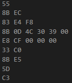
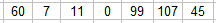
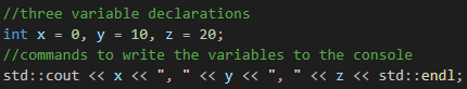

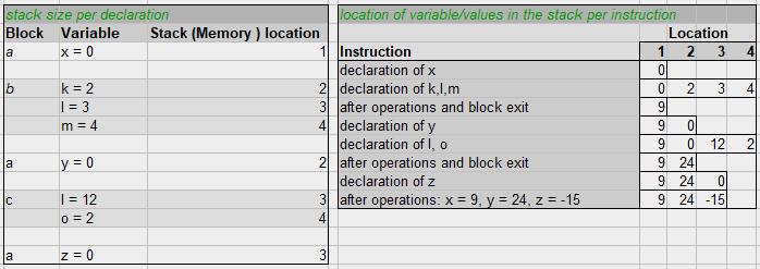

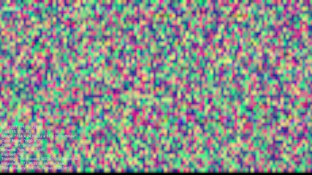
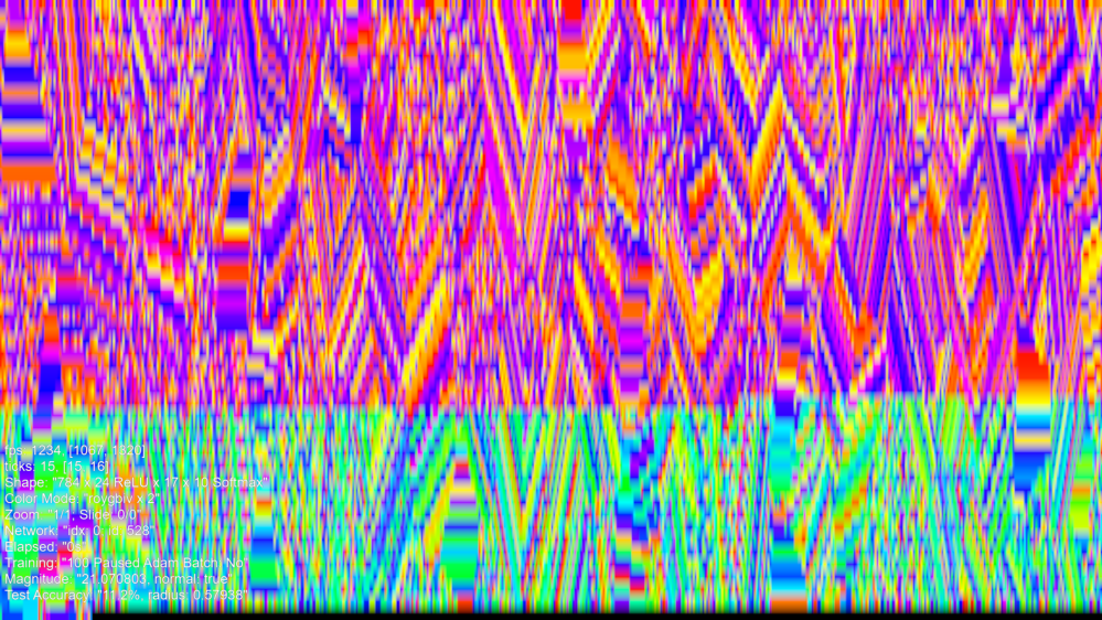
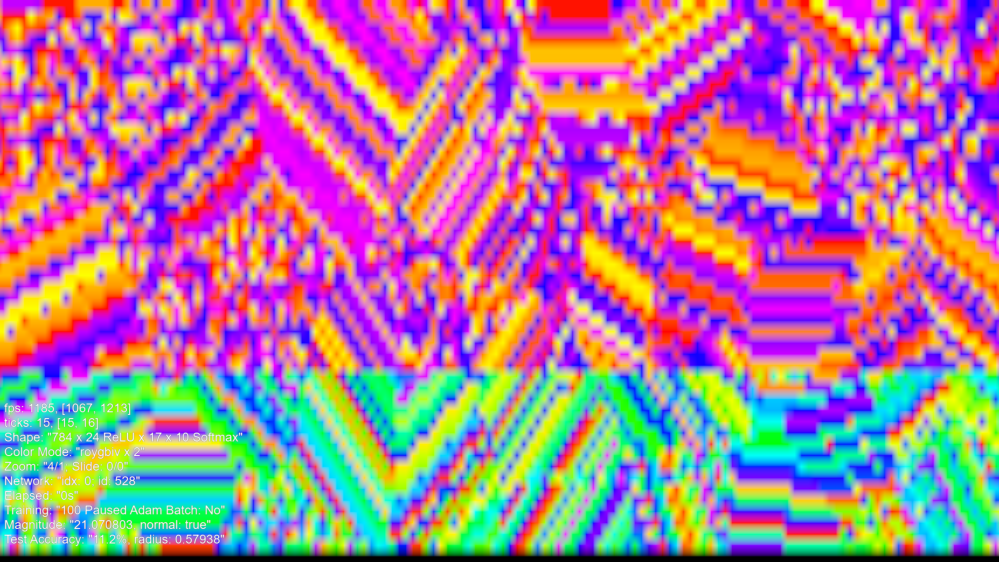
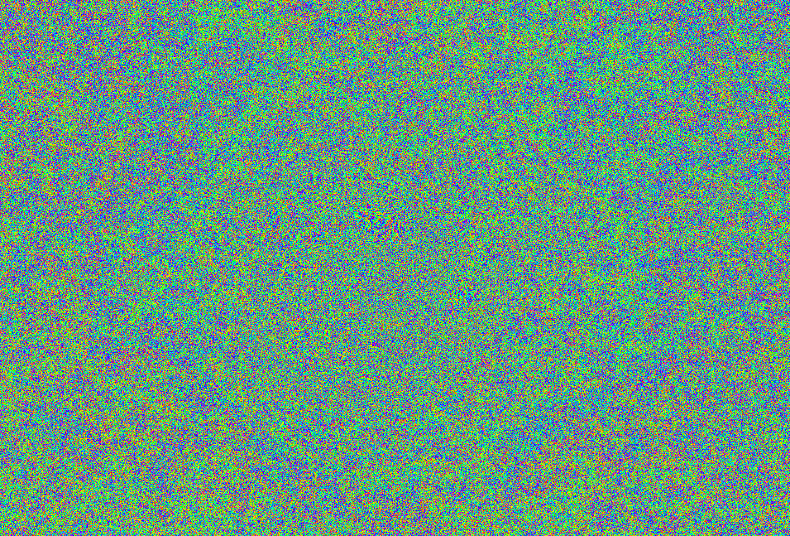
