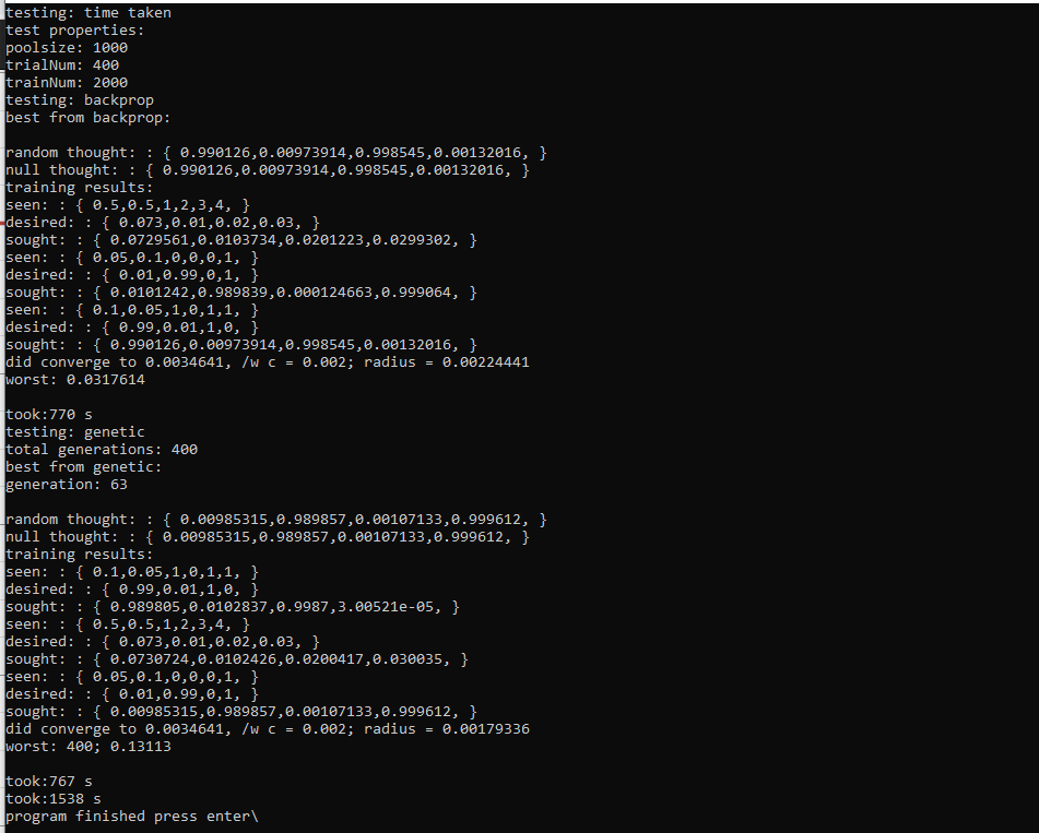
I have written an application which creates pools of 1000 neural networks. One test performs backpropagation training on them. A second test performs backpropagation, and a genetic algorithm. The amount of times training is called for each test is the same. The genetic algorithm seems to actually be able to converge on a lottery ticket and seems to always outperform backpropagation training alone.
Here is example output which will be explained:
In this example there is a total network poolsize of 1000 random networks. This network pool size is used for both the tests. To compare networks, their radius is examined, and the smaller it is, the better.
In the first test, backpropagation, the best network converges pretty well, to 0.0022~. The wost network, however, converges to 0.031~, a much worse solution. The amount of training called on the networks is constant, and yet there is a vast difference in performance based on Lottery Ticket, in a pool of just 1000 networks.
Lottery Ticket means that more ideal networks can be found and distributed periodically. The thing is, backpropagation, in its most simple form, is not a Lottery Ticket Algorithm. Genetic Algorithms are indeed a Lottery Ticket Algorithm, and it seems that backpropagation can be put into them naturally. This causes networks to evolve and change in ways that backpropagation does not even consider, for example: neuron biases. It also makes backpropagation consider itself, as it is performed socially among a pool of existent networks.
The second test is genetic. It starts from scratch with 1000 new random networks, runs for 400 generations, and calls training (backpropagation) the same amount of times as the earlier test. On generation 65, a Lotto is won for a particular network, and it ends up outperforming all others found in either tests. The amount of trainings on the winning network is the sum of its parents and the remaining trainings it did. That winning network, went into all future generations along with various other algorithm and mutations of networks. I guess I am going to consider this a Lottery Network.
What we need to do is somehow, find these networks that exist, maybe, or could, but are hard to find, and the search could never end. I think to do both backpropagation and genetic algorithms and other functions such as pruning, growth, or other mutation. What else can be used? It seems like there are likely concepts in math or other sciences which could contribute. Recently, in creating mutation functions, I applied a normal distribution function and am performing math on normal distributions, which is new to me, or what else could be available or how this should evolve is unknown.
the basic normal distribution function I’ve made looks like the following on desmos:
It is used to ‘decide’ when to mutate something and by what magnitude. Most of the time this magnitude is small and otherwise approaches one. It seems like evolutionary algorithms could be benefited with the study of probability maths or other maths and I may do this at some point.
Next is to add methods of pruning and growth to networks to further investigate Lottery Ticket.
I have been studying neural networks for some time, and recently during a YSU hackthon, I managed to make interesting progress. After about a year long break, I return to this code and make large amounts of progress and a number of topics have presented in C++ software.
I’m going to describe some of my journey into AI in C++ and talk about AI in blog format from the persepective of a modern C++ developer.
Neural networks are in concept similar to brains. What they are is a pattern processing algorithm. In typical neural networks, there are layers of patterns, each modified by the previous in sequence. When this sequence goes forward, we do something called Feed-forward, which is taking a pattern, running it through the network, and producing a pattern-deduced result. So, a network could take input images/patterns of dogs, and output whether it is a dog or not. Feed Forward can be reversed in a way through something called Back Propagation. During Back Propagation, Calculus is used to adjust the pattern’s error throughout the network. The result is training to recognize the pattern, making Feed Forward less error-prone.
This, at least, was my understanding after completing the hackthon code. What I had done during the hackthon was reference a blog-paper which describes the calculus of backpropagation and produce a seemingly functional algorithm in C++.
These sequenced Neural Networks are easily represented as series of vectors and matrices, and Feed Forward is as simple as performing maths across the series to its end, the output. Feed-forward can produce accurate results and the effect of pattern recognition. A thought is the vector result of Feed Forward for any arbitrary input. The thought about each training data represents the network’s accuracy about the training data, and is said to converge to some accuracy. Matrices may not be the best way to represent this data in light of modern Data-Oriented concepts.
In my study of Backpropagation, it seems like the Backpropagation function produces a magnitude of error. That magnitude then is used to adjust existing error. Adjusting by this magnitude does not train the network in a single iteration, (for reasons that will be explained), therefore Backpropagation is done iteratively.
One reason it is done iteratively, has to do with the initial solution surface of the network, the initial configuration. The initial configuration of the network can have beneficial or detrimental effects on how the network converges if at all. This seems problematic and so we could move the problem from training networks toward finding solution surfaces for initial or final configurations of networks. In searching vast random solution space there is an immediate ally, genetic algorithms. Backpropagation and Genetic Algorithms combine to make an error direction and ability to move across solution surfaces efficiently with averaging and bounded random movement. This sort of algorithm also scales by increasing parallel hardware, which is ideal. The question is whether there is a better way to search for ideal networks. Out of a potential infinity of vast solution space, what is the most efficient way to converge on an ideal network? How long should it take? What is the ideal network, or how could it emerge?
This leads to something called: Lottery Ticket Hypothesis. The idea goes, for a given network, there is a smaller network that converges the same or similarly. Finding this network, that is winning the lottery. The question is how to find it, and in the end: it could be easy to find, stumbled upon eventually, or entirely impossible. In the algorithm for this theory, a network is trained using backpropagation. Next, it is pruned by the least contributing factors and then trained more, in a repeated fashion. I think what must happening, is that when a least contributing factor is eliminated, existing factors must take up slack or the network will not converge.
The existence of a converging network or its ability to take up slack, depends on the numbers that can be found within it. Future computers are going to need ever better and more accurate floating-point number representation, in order to make finding these networks more likely. It is entirely possible that the existence of networks has to do about their ultimate hardware representation and they may not be very portable.
Object oriented programming is the typical go-to method of programming, and it is super useful, especially in a program’s “sculpting”/exploration or design phase. The problem with it, however, is that modern computer hardware has evolved and typical OOP practices have not. The main issues are that hardware is getting more parallelized and cache-centric. What this means is that programs benefit when they can fetch data from the catch rather than RAM, and when they can be parallelized. Typical, Object Oriented Programming, it turns out, does little to take advantage of these new hardware concepts, if indeed it does not oppose them.
Data Oriented Design is a design philosophy being popularized in video game programming, where there is a lot of opportunity for both parallelization and cache consideration. I think this concept can be useful to some extent everywhere, however, and a programmer should be aware of what it is and how to make use of it. Cache speed is enormous compared to RAM, and by default, there are absolutely no considerations about it being made by programmers. This should change. Unfortunately, a lot of popular languages, developed and evolved in the concept of infinite resources, a logical fallacy, offer little to no support for cache-centric programming (Java/.Net). Fortunately, in C++, we have future. Working with DoD is going to be beneficial until (if) computer hardware ever becomes unified and the “cache” becomes gigabytes in size. Until then, however, we must work with both RAM and Cache in our designs, if they are to be performant.
To start, lets look at typical OOP and what sort of performance characteristics it has.
First off, the simple Object and an Array of them:
class Object{
 public:
  int x, y, z;
  float a, b, c;
  int* p;
};
std::vector<Object> objects;
In this example, we have various variables composed into an object. There are several things going on here:
a) The Object is stored in a contiguous segment of memory, and when we go to reference a given variable, ( x, y, z, a, b, c, p ), the computer goes out to fetch that data, and if it is not already in the Cache, it gets it from Ram, and memory near to it, and puts it into the Cache. This is how the Cache fills up, recently referenced data and data near to it. Because the cache is limited in size, it periodically will flush segments to RAM or retrieve new segments from RAM. This read/write process is takes time. The key concept here is that it also fetches *nearby* data, anticipating that you may be planning to access it sequentially or that it may be related and soon used.
b) The variable, (p), is a pointer. When this variable is dereferenced, the cache is additionally filled by that data ( and near data) additionally. Fetching memory from a pointer may cause additional catch filling/flushing in addition to merely considering the pointer itself.
c) considering the vector: objects; objects is a contiguous segment of memory and accessing non-pointer data sequentially is ideal. When element x is referenced, so then there is a good chance that x+y and x-y elements were all stored into the cache simultaneously for speedy access. Because the vector is contiguous, all of the bytes of every object are stored in sequence. The amount of objects accessible in the Cache is going to depend on the size of the Object in bytes.
We will examine an example application comparing the performance of OOP and DOD.
To begin, lets create a more realistic OOP object to make a comparison with:
class OopObject {
public:
	Vector3 position, velocity;
	float radius;
	std::string name;
	std::chrono::steady_clock::time_point creationTime;


	void load() {

		//initialize with some random values;
		position = reals(random);
		velocity = reals(random);
		radius = reals(random);

		name = "test" + std::to_string(radius);
		creationTime = std::chrono::steady_clock::now();
	}

	void act() {
		//this is a function we call frequently on sequences of object
		position += velocity;
	}
};
We interact with this object in a typical OOP fashion, we create a vector, dimension it, loop through, initialize the elements, then we loop through again and do the “act” transform, and then we loop through again and do an “avg” calculation.
To start programming DoD, we need to consider the Cache rather than using it by happenstance. This is going to involve organizing data differently. In Object Orientation, all data is packed into the same area and therefore is always occupying cache, even if you only care about a specific variable and no others. If we are iterating over an array of objects and only accessing the same 20% of data the whole time, we are constantly filling the cache with 80% frivolous data. This leads to a new type of array and a typical DoD Object.
The first thing we do is determine what data is related and how it is often accessed or what we want to tune towards, then we group that data together in their own structures.
The next thing we do is create vectors of each of these structures. The DoDObject is in fact a sort of vector manager. Rather than having a large vector of all data, we have series of vectors with specific data. This increases the chances of related data being next to each other, while optimizing the amount that’s actually in the cache because there’s no space taken by frivolous data.
class DoDObject {
public:
struct Body {
Vector3 position, velocity;
};
struct Shape {
float radius;
};
struct Other {
std::string name;
std::chrono::steady_clock::time_point creationTime;
};
std::vector< Body > bodies;
std::vector<Shape > shapes;
std::vector<Other> others;
DoDObject(int size) {
bodies.resize(size);
shapes.resize(size);
others.resize(size);
}
void load() {
for (auto& b : bodies) {
b.position = reals(random);
b.velocity = reals(random);
}
for (auto& s : shapes) {
s.radius = reals(random);
}
int i = 0;
for (auto& o : others) {
o.name = "test" + std::to_string(shapes[i++].radius);
o.creationTime = std::chrono::steady_clock::now();
}
}
void act() {
for (auto& b : bodies) {
b.position += b.velocity;
}
}
};
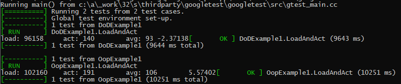
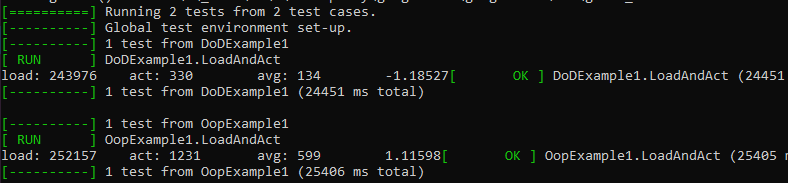
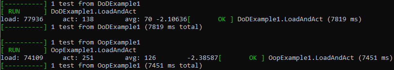
Lets look at the results, at the end will be the complete source file.
(AMD Ryzen 7 1700)
(AMD FX 4300)
(Intel(R) Core(TM) i7-4790K)
DOD has won on every test. This is a simple example program, too. Actual programs are going to see even larger gains.
Here’s the complete source of this example: (GoogleTest C++)
#include "pch.h"
#include <vector>
#include <chrono>
#include <string>
#include <random>
std::uniform_real_distribution<float> reals(-10.0f, 10.0f);
std::random_device random;
int numObjects = 100000;
struct Vector3 {
float x, y, z;
Vector3() = default;
Vector3(float v) : x(v), y(v + 1), z(v + 2) {}
Vector3& operator+=(const Vector3& other) {
x += other.x;
y += other.y;
z += other.z;
return *this;
}
};
class OopObject {
public:
Vector3 position, velocity;
float radius;
std::string name;
std::chrono::steady_clock::time_point creationTime;
void load() {
//initialize with some random values;
position = reals(random);
velocity = reals(random);
radius = reals(random);
name = "test" + std::to_string(radius);
creationTime = std::chrono::steady_clock::now();
}
void act() {
//this is a function we call frequently on sequences of object
position += velocity;
}
};
class DoDObject {
public:
struct Body {
Vector3 position, velocity;
};
struct Shape {
float radius;
};
struct Other {
std::string name;
std::chrono::steady_clock::time_point creationTime;
};
std::vector< Body > bodies;
std::vector<Shape > shapes;
std::vector<Other> others;
DoDObject(int size) {
bodies.resize(size);
shapes.resize(size);
others.resize(size);
}
void load() {
for (auto& b : bodies) {
b.position = reals(random);
b.velocity = reals(random);
}
for (auto& s : shapes) {
s.radius = reals(random);
}
int i = 0;
for (auto& o : others) {
o.name = "test" + std::to_string(shapes[i++].radius);
o.creationTime = std::chrono::steady_clock::now();
}
}
void act() {
for (auto& b : bodies) {
b.position += b.velocity;
}
}
};
template<typename Action>
void time(const std::string& caption, Action action) {
std::chrono::microseconds acc(0);
//each action will be executed 100 times
for (int i = 0; i < 100; ++i) {
auto start = std::chrono::steady_clock::now();
action();
auto end = std::chrono::steady_clock::now();
acc += std::chrono::duration_cast<std::chrono::microseconds>(end - start);
}
std::cout << caption << ": " << (acc.count() / 100) << "\t";
};
TEST(DoDExample1, LoadAndAct) {
DoDObject dod(numObjects);
time("load", [&]() {
dod.load();
});
time("act", [&]() {
dod.act();
});
float avg = 0;
time("avg", [&]() {
float avg1 = reals(random);
for (auto& o : dod.shapes) {
avg1 += o.radius;
}
avg1 /= dod.shapes.size();
avg += avg1;
});
std::cout << avg;
EXPECT_TRUE(true);
}
TEST(OopExample1, LoadAndAct) {

	std::vector<OopObject> objects;

	objects.resize(numObjects);

	time("load", [&]() {


		for (auto& o : objects) {
			o.load();
		}

		});

	time("act", [&]() {

		for (auto& o : objects) {
			o.act();
		}

		});

	float avg = 0;
	time("avg", [&]() {

		float avg1 = reals(random);

		for (auto& o : objects) {
			avg1 += o.radius;
		}

		avg1 /= objects.size();

		avg += avg1;
		});
	std::cout << avg;

	EXPECT_TRUE(true);
}
This is a continuation of an earlier post called, Division By Zero Exploration, which was a continuation of an even earlier post, Division By Zero.
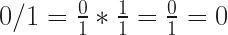
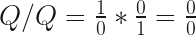
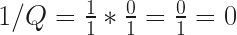
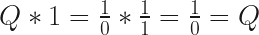
In the exploration post, I concluded that, if dividing by zero is valid, then, “it is basically possible to make anything equal anything”. Further thought has lead to an additional conclusion: one does not necessarily equal one. This becomes evident from the basic properties of Q and 0, and specifically, infinity times zero equals one, or Q*0=1. If this holds true, then one does not necessarily equal one. Here we go.
What I mean is that: one may not equal one, all the time. This is because we can rewrite Q*0 = 1 an infinite amount of ways by adding additional zeros or Qs. ( At least, if 0*0 = 0 and Q*Q=Q). The way the expression is factored causes it to have a potential series of possible answers, some true, and others false.
There are two basic expansions, each which results in two different possible outcomes, for a potential of three answers. The first is Q*0*0. If it holds true that 0*0 always equals zero, then this should be a rational procedure. This results in two possible factorings: (Q*0)*0 and Q*(0*0). The first factoring equals 1, the second equals 0. The other basic expansion is Q*Q*0. This ends up resulting in either 1 or Q.
When we add in the x variable, Q*0*X, we get outcomes 1 or X.
Using this process, I go back to the previous example of a=b and start with a+b=b. From here, there are a lot of potential procedures, but the simplest path to a=b is two steps, I think.
Q*0*b resolves to 1 which resolves to Q*0*0
Q*0*0 resolves to 0
Of course, there are other outcomes from this procedure that are false. These are the other generated outcomes:
This leads to another conclusion,zero does not necessarily equal zero, nor does Q equal Q.
I think inventing math is my new hobby, comments are appreciated.
C++ 17 has Structured Bindings, what they do is create a temporary object and provide access to the object’s members locally.
struct S{
    int a{5};
    float b{3.2};
};

auto [x,y] = S();
What happens is we create a temporary S object, and then copy the values memberwise into the binding structure. x now equals 5 and b equals 3.2. the S instance goes away.
Since functions only can return one value normally, to get additional values out, we use by-reference variables.
void f( int& a, float& b ){
    a = 10; b = 3.2f;
}
This leads to a programming style where we do two things:
create variables to hold the return values before the call
pass the variable to the function as a parameter.
int x=0;
float y=0;
f( x, y );
//x == 10; y = 3.2f;
It has never been glancingly apparent that the values are not only being passed by reference, which is often the case for performance, but they are also output from the function with changed values.
Structured Bindings provides a solution to this potential issue:
auto f(){
    int a{10};
    float b{3.2f};

    return std::make_tuple(a,b);
}

auto [x,y] = f();
Since tuples can have as many parameters as we want, they are an easy way to accomplish creating the return structure for the binding.
In C++11 there is a less effective way to do return type Binding:
int x; float y;
std::tie( x, y ) = f();
Structured Bindings also works with arrays, and can be used to create variable aliases as well.
auto f(){
    int a{10};
    float b{3.2f};

    return std::make_tuple(a,b);
}

auto f2( const int& i ){
    return std::make_tuple(std::ref(i));
}

auto [x, y] = f();

auto [r] = f2(x);

++x;

x = r + 1;
//r is a reference to x, x = 12
This does not mean that by-reference should never be used – it should be where appropriate. What it means is that if a variable is just a return argument, and not also a function argument, then maybe it should be passed out via a Structured Binding and not passed in by reference.
I discovered a GDC talk on a topic called: Asymptotic Averaging. This is sort of a form of interpolation, and can be used to eliminate jerky motions – in particular, they focus on camera movement. Naturally, when you want to change a camera’s direction, you just set the direction. However, if you are doing this frequently or if the distance is large, it results in a jerk or jump which can be disorienting to some extent. This is demonstrated easily by having a camera follow a player character.
Here’s a video of a jerky camera from my current project:
Asymptotic means always approaching a destination but never reaching it. In math it occurs as a curve approaches an asymptote but never actually reaches it. Besides being easy to implement, we get a curve to our movement as well.
The easy to implement concept is from the following form:
In this variation we are working with a translation. What happens is offsetPosition is set to the translation offset (dest-current). Then each update (frame) we call reduce, which returns a smaller amount of the translation to perform each time. This translation continues to shrink and approaches zero.
Using variations of this, it is easy to produce Trailing and Leading Asymptotic Movement.
Here’s a vid of Trailing Camera Rotation + Trailing Camera Movement:
Here’s a vid of Leading Camera Rotation + Trailing Camera Movement:
C++17 has a powerful template feature – Fold Expressions – that combines with a C++11 feature – Parameter Pack. This allows us to do away with C-style variable arguments (variadic functions). I introduce Lamda Overloading as well, to work with these two concepts in a wonderful way.
First off, the Parameter Pack. This is a template feature that allows a variable amount of parameters to be passed to the template. Here’s a sum function declaration:
template<typename ...Args>
auto sum(Args... args);
In the template area, there are a variable amount of parameters, called Args. In the function area, the arguments accepted are the various parameters, Args. Each element in that pack of parameters will be referred to as, args, inside the function body.
A fold is contained within parenthesis. Sequentially, left most parameters to right most are included, each called args. Next, each specific parameter, each args, is combined with some operator, in this case, addition. Finally, ellipses signals repeat for each arg.
int i = sum(0,3,5);
Expands to the following, at compile-time:
return (0 + 3 + 5);
So what we’re going to do is write a more modern printf sort of function without using a c variadic function. There are a lot of ways to do this, but because I love lamdas, I want to include lamdas as well. Here we go:
So, in order to vary the generation of strings based on the type of the input parameter, at compile-time, we need to use additional templates. The first thing necessary was an ability to do function overloading with lamdas, hence the LamdaOverload class. This class basically incorporates a bunch of lamdas under one name and overloads the execution operator for each one.
Next, inside the new_printf function, we define the deduce LamdaOverload object. This object is used to define routes from data types to code-calling. There are different types accepted, and one is a catch-all type which is going to be used for natives that work with the std::to_string function. Note that if the catch-all doesn’t work with std::to_string, an error will be generated.
You can add more overloads to LamdaOverload to accept custom types as well. For instance,
[](const MyClass& c) ->std::string { return c.toString(); }
The call ends up looking like so:
new_printf("the value of x: ", int(x), std::string("and"), 0.1f );
This post isn’t so much about programming as much about an earlier post about Division By Zero. So, I thought, if the reciprocal operation to 1 / 0,0 / 1, is valid, then maybe division by zero can be postponed and considered later. Similar to the imaginary concept, i or sqrt(-1).
Using just fraction concepts I managed to accomplish a lot of progress and, not being a mathematician, I don’t know how much merit there is to it, but here we go.
First, the assumptions:
OK, so now something that I found immediately useful to do with Q and seems to make sense, furthermore this is what lead me to think up Q.
Consider the following:
True, 0 = 0; now considering the reciprocal:
how does this resolve?
What this leads to is another assumption: algebraically, the same way Q can be considered for later, so then, can Zero be considered later.
Consider:
distribute zero once and then multiply both sides by Q (divide by zero )
Now – I realize – if I had distributed the zero to the a instead, the answer would have come out incorrect.
Once it is possible to divide by zero and turn a zero into a one, it seems like it’s possible to produce lots of wrong answers, but some correct ones as well, it seems like it depends on trial and error, perhaps, or additional processing of some sort.
So, I’ve been messing around with this concept using my limited math skills, and it seems like sometimes Q works, and sometimes, it doesn’t work. It’s like sometimes there’s a good solution and an infinity of wrong ones, or the opposite, or some mix of random, maybe. I just don’t know. At the end of the day, sometimes it works, so maybe there is merit.
What I’ve concluded is that with this concept, a consequence, is that it’s possible to basically make anything equal anything, and that seems like an odd thing to consider.
I wanted to quickly create a thread pooler that could be passed lamdas. Turns out it’s super simple. Here are the main things I wanted to accomplish:
pass lamdas as tasks to be executed asap.
be able to wait for all tasks to execute
create a bunch of threads at initialization and them have then wait around for tasks, since it can be time-costly to create a new thread on the fly.
be able to create as many poolers as I want for different uses.
The first thing I needed to be able to do was store a bunch of lamdas in a single vector, and any sort of lamda. I decided the easiest way to do this was to use lamda members for the task parameters. This is what add task call could look like:
int x, y,z;

mThreadPool.addTask([x,y,z](){
    //task on x, y, z ...
});
The task should execute on another thread as soon as possible.
So in a loop, I’d call, mThreadPool.addTask a bunch of times, and then I’d have to wait on them like so:
mThreadPool.wait();
To store the task lamdas inside the ThreadPool, I used an std::function:
This works because the task receives its parameters from the lamda itself, not from the lamda call operator. There has to be a mutex because multiple threads are going to query the mTasks vector.
I wanted to create the entire thread pool at one time, so there are initialize and shutdown functions:
The number of tasks currently executing is kept track of with mTasksExecutingCount. When the ThreadPool is waiting, it waits until the count is zero and the mTasks.size is zero.
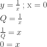
So we all know that dividing by zero is an error in programming, but do you know why?
It turns out that it not really an error as much as a math problem, and not so much a problem as much as a thing. Here’s how it goes according to my understanding:
A function y= 1 * x has a domain of all real numbers
A function y= 1 / x has a domain of x != 0, zero is an asymptote
If you look at the graph of the function, y = 1 / x, and you think about it, 1 / x approaches infinity as x moves toward zero, but it never actually reaches zero. Obviously we can conceive to write, y = 1 / 0, but as an actual operation, it doesn’t make sense as 0 is outside the domain of 1 / x. Why it is outside the domain of x, I’m not entirely sure, but it is, and that’s how it is. At the end of the day, it seems that x=0 and y= 1 / x each draw a separate, non-intersecting line.
If the C++ compiler detects that you’ve done a/ 0, it will consider it undefined behavior, and make the entire thing a no-op. If it makes it a no-op, it may not tell you, and this could be a source of a bug. If you encounter a/0 during run-time, you may get some sort of crash or exception.
With the way the compiler can optimize, it can reorder some source operations to affect performance. It’s possible for the compiler to place a divide by zero error before a statement you need or would expect to be executed. You would experience undefined behavior ( x / 0 ) at a place that is not indicated via source code, and that’s bad.